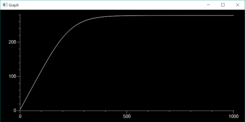
Temperature change over time (in thousands of years). As the Earth warms from 3K to equilibrium.
If the Earth behaved as a perfect black body and absorbed all incoming solar radiation (and radiated with 100% emissivity) the we calculated that the average surface temperature would be about 7 degrees Celsius above freezing (279 K). Keeping with this simplification we can think about how the Earth’s temperature could change with time if it was not at equilibrium.
If the Earth started off at the universe’s background temperature of about 3K, how long would it take to get up to the equilibrium temperature?
Using the same equations for incoming solar radiation (Ein) and energy radiated from the Earth (Eout):
At equilibrium the energy in is equal to the energy out, but if the temperature is 3K instead of 279K the outgoing radiation is going to be a lot less than at equilibrium. This means that there will be more incoming energy than outgoing energy and that energy imbalance will raise the temperature of the Earth. The energy imbalance (ΔE) would be:
All these energies are in Watts, which as we’ll recall are equivalent to Joules/second. In order to change the temperature of the Earth, we’ll need to know the specific heat capacity (cE) of the planet (how much heat is required to raise the temperature by one Kelvin per unit mass) and the mass of the planet. We’ll approximate the entire planet’s heat capacity with that of one of the most common rocks, granite. The mass of the Earth (mE) we can get from NASA:
cE = 800 J/kg/K
mE = 5.9723×1024kg
So looking at the units we can figure out the the change in temperature (ΔT) is:
Where Δt is the time step we’re considering.
Now we can write a little program to model the change in temperature over time:
EnergyBalance.py
from visual import *
from visual.graph import *

I = 1367.
r_E = 6.371E6
c_E = 800.
m_E = 5.9723E24

sigma = 5.67E-8

T = 3                               # initial temperature

yr = 60*60*24*365.25
dt = yr * 100
end_time = yr * 1000000
nsteps = int(end_time/dt)

Tgraph = gcurve()

for i in range(nsteps):
    t = i*dt
    E_in = I * pi * r_E**2
    E_out = sigma * (T**4) * 4 * pi * r_E**2
    dE = E_in - E_out
    dT = dE * dt / (c_E * m_E)
    T += dT
    Tgraph.plot(pos=(t/yr/1000,T))
    if i%10 == 0:
        print t/yr, T
        rate(60)
The results of this simulation are shown at the top of this post.
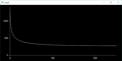
What if we changed the initial temperature from really cold to really hot? When the Earth formed from the accretionary disk of the solar nebula the surface was initially molten. Let’s assume the temperature was that of molten granite (about 1500K).
Cooling if the Earth started off molten (1500K). Note that this simulation only runs for 250,000 years, while the warming simulation (top of page) runs for 1,000,000 years.
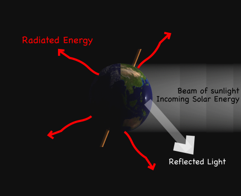
For conservation of energy, the short-wave solar energy absorbed by the Earth equals the long-wave outgoing radiation.
Energy and matter can’t just disappear. Energy can change from one form to another. As a thrown ball moves upwards, its kinetic energy of motion is converted to potential energy due to gravity. So we can better understand systems by studying how energy (and matter) are conserved.
Energy Balance for the Earth
Let’s start by considering the Earth as a simple system, a sphere that takes energy in from the Sun and radiates energy off into space.
Incoming Energy
At the Earth’s distance from the Sun, the incoming radiation, called insolation, is 1367 W/m2. The total energy (wattage) that hits the Earth (Ein) is the insolation (I) times the area the solar radiation hits, which is the area a cross section of the Earth (Acx).
Given the Earth’s radius (rE) and the area of a circle, this becomes:
Outgoing Energy
The energy radiated from the Earth is can be calculated if we assume that the Earth is a perfect black body–a perfect absorber and radiatior of Energy (we’ve already been making this assumption with the incoming energy calculation). In this case the energy radiated from the planet (Eout) is proportional to the fourth power of the temperature (T) and the surface area that is radiated, which in this case is the total surface area of the Earth (Asurface):
The proportionality constant (σ) is: σ = 5.67 x 10⁻⁸ W m-2 K-4
Note that since σ has units of Kelvin then your temperature needs to be in Kelvin as well.
Putting in the area of a sphere we get:
Balancing Energy
Now, if the energy in balances with the energy out we are at equilibrium. So we put the equations together:
cancelling terms on both sides of the equation gives:
and solving for the temperature produces:
Plugging in the numbers gives an equilibrium temperature for the Earth as:
T = 278.6 K
Since the freezing point of water is 273K, this temperature is a bit cold (and we haven’t even considered the fact that the Earth reflects about 30% of the incoming solar radiation back into space). But that’s the topic of another post.
On this year’s trip to the Current River with the Middle School we were able to see outcrops of the three major types of rocks: igneous, metamorphic, and sedimentary.
Igneous Rocks
Beautiful, pink granite at Elephant Rocks State Park.
We stopped by Elephant Rocks State Park on the way down to the river to check out the gorgeous pink granite that makes up the large boulders. The coarse grains of quartz (translucent) interbedded with the pink orthoclase crystals make for an excellent example of a slow-cooling igneous rock.
Metamorphic Rocks
The Prairie Creek waterfall pool.
On the second day out on the canoes we clambered up the rocks in the Prairie Creek valley to see jump into the small waterfall pool. The rocks turned out to look a lot like the granite of Elephant Rocks if the large crystals had been heated up and deformed plastically. This initial stage of the transformation allowed me to talk about metamorphic rocks althought we’ll see some much more typical samples when we get back to the classroom.
Prairie Creek rocks.
Sedimentary Rocks
Limestone bluffs along the Current River.
We visited a limestone cave on the third day, although we’ve been canoeing through a lot of limestone for on the previous two days. This allowed us to talk about sedimentary rocks: their formation in the ocean and then uplift via tectonic collisions.
The Rock Cycle
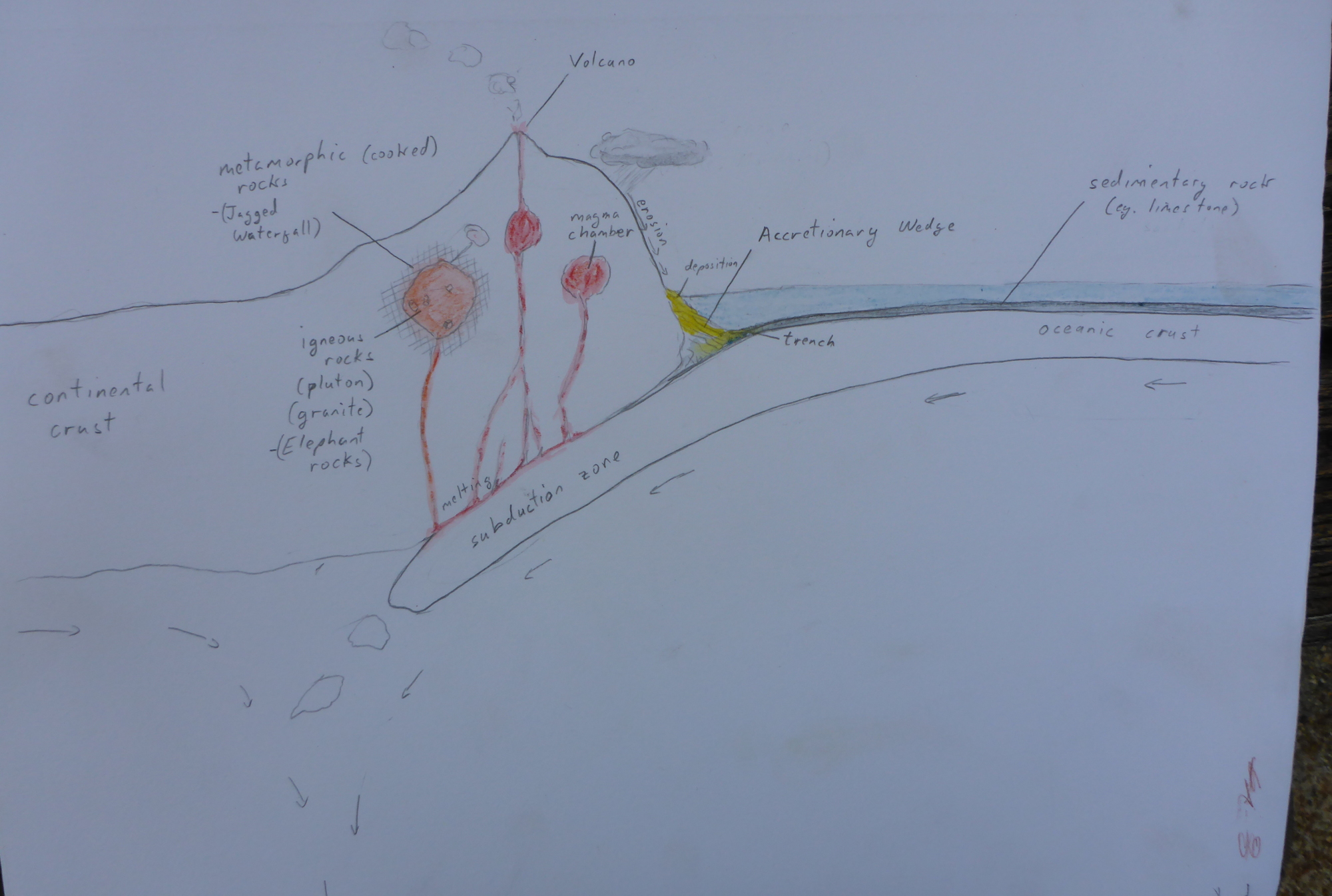
Diagram of a convergent tectonic margin used to illustrate the rock cycle.
Back at camp, we summarized what we saw with a discussion of the rock cycle, using a convergent plate margin as an example. Note: sleeping mats turned out to be excellent models for converging tectonic plates.
Note to self: It might make sense to add extra time at the beginning and end of the trip to do some more geology stops. Johnson Shut-Inns State Park is between Elephant Rocks and Eminence, and we saw a lot of interesting sedimentary outcrops on the way back to school as we headed up to Rolla.
Genetic algorithm trying to find a series of four mathematical operations (e.g. -3*4/7+9) that would result in the number 42.
I’m teaching a numerical methods class that’s partly an introduction to programming, and partly a survey of numerical solutions to different types of problems students might encounter in the wild. I thought I’d look into doing a session on genetic algorithms, which are an important precursor to things like networks that have been found to be useful in a wide variety of fields including image and character recognition, stock market prediction and medical diagnostics.
The ai-junkie, bare-essentials page on genetic algorithms seemed a reasonable place to start. The site is definitely readable and I was able to put together a code to try to solve its example problem: to figure out what series of four mathematical operations using only single digits (e.g. +5*3/2-7) would give target number (42 in this example).
The procedure is as follows:
Initialize: Generate several random sets of four operations,
Test for fitness: Check which ones come closest to the target number,
Select: Select the two best options (which is not quite what the ai-junkie says to do, but it worked better for me),
Mate: Combine the two best options semi-randomly (i.e. exchange some percentage of the operations) to produce a new set of operations
Mutate: swap out some small percentage of the operations randomly,
Repeat: Go back to the second step (and repeat until you hit the target).
And this is the code I came up with:
genetic_algorithm2.py
''' Write a program to combine the sequence of numbers 0123456789 and
    the operators */+- to get the target value (42 (as an integer))
'''

'''
Procedure:
    1. Randomly generate a few sequences (ns=10) where each sequence is 8
       charaters long (ng=8).
    2. Check how close the sequence's value is to the target value.
        The closer the sequence the higher the weight it will get so use:
            w = 1/(value - target)
    3. Chose two of the sequences in a way that gives preference to higher
       weights.
    4. Randomly combine the successful sequences to create new sequences (ns=10)
    5. Repeat until target is achieved.

'''
from visual import *
from visual.graph import *
from random import *
import operator

# MODEL PARAMETERS
ns = 100
target_val = 42 #the value the program is trying to achieve
sequence_length = 4  # the number of operators in the sequence
crossover_rate = 0.3
mutation_rate = 0.1
max_itterations = 400


class operation:
    def __init__(self, operator = None, number = None, nmin = 0, nmax = 9, type="int"):
        if operator == None:
            n = randrange(1,5)
            if n == 1:
                self.operator = "+"
            elif n == 2:
                self.operator = "-"
            elif n == 3:
                self.operator = "/"
            else:
                self.operator = "*"
        else:
            self.operator = operator

        if number == None:
            #generate random number from 0-9
            self.number = 0
            if self.operator == "/":
                while self.number == 0:
                    self.number = randrange(nmin, nmax)
            else:
                self.number = randrange(nmin, nmax)
        else:
            self.number = number
        self.number = float(self.number)

    def calc(self, val=0):
        # perform operation given the input value
        if self.operator == "+":
            val += self.number
        elif self.operator == "-":
            val -= self.number
        elif self.operator == "*":
            val *= self.number
        elif self.operator == "/":
            val /= self.number
        return val


class gene:

    def __init__(self, n_operations = 5, seq = None):
        #seq is a sequence of operations (see class above)
        #initalize
        self.n_operations = n_operations

        #generate sequence
        if seq == None:
            #print "Generating sequence"
            self.seq = []
            self.seq.append(operation(operator="+"))  # the default operation is + some number
            for i in range(n_operations-1):
                #generate random number
                self.seq.append(operation())

        else:
            self.seq = seq

        self.calc_seq()

        #print "Sequence: ", self.seq
    def stringify(self):
        seq = ""
        for i in self.seq:
            seq = seq + i.operator + str(i.number)
        return seq

    def calc_seq(self):
        self.val = 0
        for i in self.seq:
            #print i.calc(self.val)
            self.val = i.calc(self.val)
        return self.val

    def crossover(self, ingene, rate):
        # combine this gene with the ingene at the given rate (between 0 and 1)
        #  of mixing to create two new genes

        #print "In 1: ", self.stringify()
        #print "In 2: ", ingene.stringify()
        new_seq_a = []
        new_seq_b = []
        for i in range(len(self.seq)):
            if (random() < rate): # swap
                new_seq_a.append(ingene.seq[i])
                new_seq_b.append(self.seq[i])
            else:
                new_seq_b.append(ingene.seq[i])
                new_seq_a.append(self.seq[i])

        new_gene_a = gene(seq = new_seq_a)
        new_gene_b = gene(seq = new_seq_b)

        #print "Out 1:", new_gene_a.stringify()
        #print "Out 2:", new_gene_b.stringify()

        return (new_gene_a, new_gene_b)

    def mutate(self, mutation_rate):
        for i in range(1, len(self.seq)):
            if random() < mutation_rate:
                self.seq[i] = operation()


def weight(target, val):
    if val <> None:
        #print abs(target - val)
        if abs(target - val) <> 0:
            w = (1. / abs(target - val))
        else:
            w = "Bingo"
            print "Bingo: target, val = ", target, val
    else:
        w = 0.
    return w

def pick_value(weights):
    #given a series of weights randomly pick one of the sequence accounting for
    # the values of the weights

    # sum all the weights (for normalization)
    total = 0
    for i in weights:
        total += i

    # make an array of the normalized cumulative totals of the weights.
    cum_wts = []
    ctot = 0.0
    cum_wts.append(ctot)
    for i in range(len(weights)):
        ctot += weights[i]/total
        cum_wts.append(ctot)
    #print cum_wts

    # get random number and find where it occurs in array
    n = random()
    index = randrange(0, len(weights)-1)
    for i in range(len(cum_wts)-1):
        #print i, cum_wts[i], n, cum_wts[i+1]
        if n >= cum_wts[i] and n < cum_wts[i+1]:

            index = i
            #print "Picked", i
            break
    return index

def pick_best(weights):
    # pick the top two values from the sequences
    i1 = -1
    i2 = -1
    max1 = 0.
    max2 = 0.
    for i in range(len(weights)):
        if weights[i] > max1:
            max2 = max1
            max1 = weights[i]
            i2 = i1
            i1 = i
        elif weights[i] > max2:
            max2 = weights[i]
            i2 = i

    return (i1, i2)


# Main loop
l_loop = True
loop_num = 0
best_gene = None

##test = gene()
##test.print_seq()
##print test.calc_seq()

# initialize
genes = []
for i in range(ns):
    genes.append(gene(n_operations=sequence_length))
    #print genes[-1].stringify(), genes[-1].val


f1 = gcurve(color=color.cyan)

while (l_loop and loop_num < max_itterations):
    loop_num += 1
    if (loop_num%10 == 0):
        print "Loop: ", loop_num

    # Calculate weights
    weights = []
    for i in range(ns):
        weights.append(weight(target_val, genes[i].val))
        # check for hit on target
        if weights[-1] == "Bingo":
            print "Bingo", genes[i].stringify(), genes[i].val
            l_loop = False
            best_gene = genes[i]
            break
    #print weights

    if l_loop:

        # indicate which was the best fit option (highest weight)
        max_w = 0.0
        max_i = -1
        for i in range(len(weights)):
            #print max_w, weights[i]
            if weights[i] > max_w:
                max_w = weights[i]
                max_i = i
        best_gene = genes[max_i]
##        print "Best operation:", max_i, genes[max_i].stringify(), \
##              genes[max_i].val, max_w
        f1.plot(pos=(loop_num, best_gene.val))


        # Pick parent gene sequences for next generation
        # pick first of the genes using weigths for preference
##        index = pick_value(weights)
##        print "Picked operation:  ", index, genes[index].stringify(), \
##              genes[index].val, weights[index]
##
##        # pick second gene
##        index2 = index
##        while index2 == index:
##            index2 = pick_value(weights)
##        print "Picked operation 2:", index2, genes[index2].stringify(), \
##              genes[index2].val, weights[index2]
##

        (index, index2) = pick_best(weights)

        # Crossover: combine genes to get the new population
        new_genes = []
        for i in range(ns/2):
            (a,b) = genes[index].crossover(genes[index2], crossover_rate)
            new_genes.append(a)
            new_genes.append(b)

        # Mutate
        for i in new_genes:
            i.mutate(mutation_rate)


        # update genes array
        genes = []
        for i in new_genes:
            genes.append(i)


print
print "Best Gene:", best_gene.stringify(), best_gene.val
print "Number of iterations:", loop_num
##
When run, the code usually gets a valid answer, but does not always converge: The figure at the top of this post shows it finding a solution after 142 iterations (the solution it found was: +8.0 +8.0 *3.0 -6.0). The code is rough, but is all I have time for at the moment. However, it should be a reasonable starting point if I should decide to discuss these in class.
A couple new article relevant to our study of Earth History.
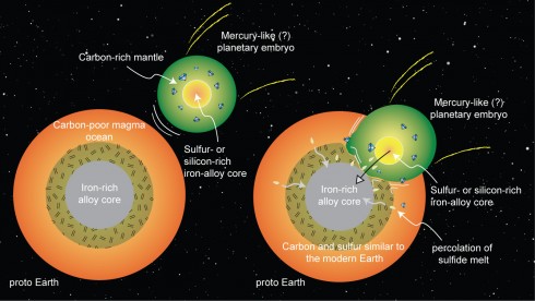
Carbon
Image by Rajdeep Dasgupta, via pyhs.org.
Research on the high pressure and temperature conditions at the Earth’s core suggest that most of the carbon in the early Earth should have either boiled off into space or been trapped by the iron in the core. So where did all the carbon necessary for life come from? They suggest from the collision of an embryonic planet (with lots of carbon in its upper layers) early in the formation of the solar system.
Free Oxygen
Typical surface view of purple mat surface at Middle Island showing purple filaments. Some white filaments can also be observed. Image from Thunder Bay Sinkholes 2008 via oceanexplorer.noaa.gov.
It took a few billion years from the evolution of the first photosynthetic cyanobacteria to the time when there was enough oxygen in the atmosphere to support animal life like us. Why did it take so long? NPR interviews scientists investigating purple microbial mats in Lake Huron.