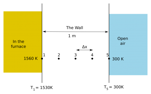
Say, for example, we have a furnace with an interior temperature of 1560 K (hot enough to melt copper) while the outside temperature is a balmy 300 K (27 Celcius). The wall of the furnace is 1 meter thick (it’s a big furnace). Can we figure out how the temperature changes inside the wall as goes from hot on the inside to cool on the outside?

To start with, we’ll look at the temperature at five points (call them nodes): three are in the wall and two at the edges (see Figure 1). We’ll say the temperature at node 1 which is next to the furnace is T1, and the temperature at the outer edge of the wall is the 5th node (T5) so:
- T1 = 1560 K
- T5 = 300 K
Now we need to find the temperature at nodes 2, 3, and 4.
Heat Flow at Equilibrium
For each of the interior nodes, we can consider how things are at equilibrium. Heat is always moving through the wall, but as some point in time the heat flowing from the furnace into the wall will be equal to the heat flowing out of the wall, and for each node the heat flowing in will equal the heat flowing out.
The heat flow (Q) from one location to another is driven by the difference in temperature (ΔT): heat flows from high temperature to cooler temperatures (which makes ΔT negative). However, you also need to consider the distance the heat is traveling (Δx) since, given the same temperature drop, heat will flow faster if the distance is short. So, it’s best to consider the temperature gradient, which is how fast the temperature is changing over distance:
![]()
How fast heat flows is also mediated by the type of material (different materials have different thermal conductivities (K)), so our heat flow equation is given by the equation:
![]()
Consider Node 2
HEAT IN: Heat is flowing into Node 2 from Node 1, so:
![]()
HEAT OUT: Heat flows out to Node 3 so:
![]()
At equilibrium the heat into the node equals the heat out:
![]()
so:
![]()
Which we can simplify a lot because we’re assuming the thermal conductivity of the wall material is constant and we’ve (conveniently) made the spacing between our nodes (Δx) the same. Therefore:
![]()
And now we solve for temperature at T2 to get:
![]()
Finally, we can break the fraction into separate terms (we need to do this to make it easier to solve using matricies as you’ll see later) and start using decimals.
![]()
If we do the same for all the internal nodes we get:
![]()
![]()
You should be able to see here that the temperature at each node depends on the temperature of the nodes next to it, and we can’t directly solve this because we don’t know the temperatures of the interior nodes.
A System of Equations
Let’s collect all of our information to get a system of equations:
- T1 = 1560 K
- T2 = 0.5 T1 + 0.5 T3
- T3 = 0.5 T2 + 0.5 T4
- T4 = 0.5 T3 + 0.5 T5
- T5 = 300 K
Now to rewrite this as a matrix. We start by putting all terms with variables on the left and all the constants on the right.
- T1 = 1560 K
- -0.5 T1 + T2 – 0.5 T3 = 0
- -0.5 T2 + T3 – 0.5 T4 = 0
- -0.5 T3 + T4 – 0.5 T5 = 0
- T5 = 300 K
Now to matrixize:

This you can solve on paper, and, if you’d like, check your answer using Alex Shine’s Gaussian Elimination solver, which gives step by step output (although it’s a little hard to follow). I used Alex’s solver to get the result:
Solution
Variable 1 = 1560.0
Variable 2 = 1245.0
Variable 3 = 930.0
Variable 4 = 615.0
Variable 5 = 300.0
This problem is set up to be easy to check because the results should be linear (if you plot temperature versus distance through the wall you’ll get a straight line). It will also give you whole number results up to 10 nodes.
Next Steps
Any Number of Nodes
This procedure for setting up the matrix give the same basic equations no matter how many nodes you use, because as long as the distance between the nodes (Δx) and the thermal conductivity (K) are constant, the equation for each internal node (Ti) will be:
[math] T_i = \frac{T_{i-1} + T_{i+1}}{2}
and the matrix will continue to just have three terms along the diagonal.
Non-uniform Wall and Non-uniform Node Spacing
If the wall is not uniform then the thermal conductivity coefficient does not just drop out of the equation, so you’ll have to pay attention to the conductivity going into and out of each node. Same goes with the node spacing.
Alternative Solution Methods
Students could try:
- writing their own matrix solvers.
- setting up the system of equations in a spreadsheet program (they’ll need to change your program’s settings so that it uses its iterative solver).