Stepper motors are used for high precision motion, like that needed for 3d printers and CNC machines. The Learn Engineering channel on YouTube explains how they work.
Tag: physics
The Physics of GPS
A nice explanation, from the excellent Real Engineering channel, of the physics of GPS that explains how the satellites must adjust for the effects of special and general relativity.
Modeling Earth’s Energy Balance (Zero-D) (Transient)
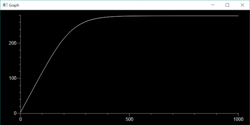
If the Earth behaved as a perfect black body and absorbed all incoming solar radiation (and radiated with 100% emissivity) the we calculated that the average surface temperature would be about 7 degrees Celsius above freezing (279 K). Keeping with this simplification we can think about how the Earth’s temperature could change with time if it was not at equilibrium.
If the Earth started off at the universe’s background temperature of about 3K, how long would it take to get up to the equilibrium temperature?
Using the same equations for incoming solar radiation (Ein) and energy radiated from the Earth (Eout):


Symbols and constants are defined here except:
- rE = 6.371 x 10⁶ m
At equilibrium the energy in is equal to the energy out, but if the temperature is 3K instead of 279K the outgoing radiation is going to be a lot less than at equilibrium. This means that there will be more incoming energy than outgoing energy and that energy imbalance will raise the temperature of the Earth. The energy imbalance (ΔE) would be:

All these energies are in Watts, which as we’ll recall are equivalent to Joules/second. In order to change the temperature of the Earth, we’ll need to know the specific heat capacity (cE) of the planet (how much heat is required to raise the temperature by one Kelvin per unit mass) and the mass of the planet. We’ll approximate the entire planet’s heat capacity with that of one of the most common rocks, granite. The mass of the Earth (mE) we can get from NASA:
- cE = 800 J/kg/K
- mE = 5.9723×1024kg
So looking at the units we can figure out the the change in temperature (ΔT) is:

Where Δt is the time step we’re considering.
Now we can write a little program to model the change in temperature over time:
EnergyBalance.py
from visual import *
from visual.graph import *

I = 1367.
r_E = 6.371E6
c_E = 800.
m_E = 5.9723E24

sigma = 5.67E-8

T = 3                               # initial temperature

yr = 60*60*24*365.25
dt = yr * 100
end_time = yr * 1000000
nsteps = int(end_time/dt)

Tgraph = gcurve()

for i in range(nsteps):
    t = i*dt
    E_in = I * pi * r_E**2
    E_out = sigma * (T**4) * 4 * pi * r_E**2
    dE = E_in - E_out
    dT = dE * dt / (c_E * m_E)
    T += dT
    Tgraph.plot(pos=(t/yr/1000,T))
    if i%10 == 0:
        print t/yr, T
        rate(60)
The results of this simulation are shown at the top of this post.
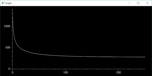
What if we changed the initial temperature from really cold to really hot? When the Earth formed from the accretionary disk of the solar nebula the surface was initially molten. Let’s assume the temperature was that of molten granite (about 1500K).
Maximum Range of a Potato Gun
One of the middle schoolers built a potato gun for his math class. He was looking a the mathematical relationship between the amount of fuel (hair spray) and the hang-time of the potato. To augment this work, I had my Numerical Methods class do the math and create analytical and numerical models of the projectile motion.
One of the things my students had to figure out was what angle would give the maximum range of the projectile? You can figure this out analytically by finding the function for how the horizontal distance (x) changes as the angle (theta) changes (i.e. x(theta)) and then finding the maximum of the function.

Distance as a function of the angle
In a nutshell, to find the distance traveled by the potato we break its initial velocity into its x and y components (vx and vy), use the y component to find the flight time of the projectile (tf), and then use the vx component to find the distance traveled over the flight time.
Starting with the diagram above we can separate the initial velocity of the potato into its two components using basic trigonometry:

 ,
,
so,
 ,
,

Now we know that the height of a projectile (y) is given by the function:

(you can figure this out by assuming that the acceleration due to gravity (a) is constant and acceleration is the second differential of position with respect to time.)
To find the flight time we assume we’re starting with an initial height of zero (y0 = 0), and that the flight ends when the potato hits the ground which is also at zero ((yt = 0), so:


Factoring out t gives:

Looking at the two factors, we can now see that there are two solutions to this problem, which should not be too much of a surprise since the height equation is parabolic (a second order polynomial). The solutions are when:


The first solution is obviously the initial launch time, while the second is going to be the flight time (tf).


You might think it’s odd to have a negative in the equation, but remember, the acceleration is negative so it’ll cancel out.
Now since we’re working with the y component of the velocity vector, the initial velocity in this equation (v0) is really just vy:

so we can substitute in the trig function for vy to get:

Our horizontal distance is simply given by the velocity in the x direction (vx) times the flight time:

which becomes:

and substituting in the trig function for vx (just to make things look more complicated):

and factoring out some of the constants gives:

Now we have distance as a function of the launch angle.
We can simplify this a little by using the double-angle formula:

to get:

Finding the maximum distance
How do we find the maxima for this function. Sketching the curve should be easy enough, but because we know a little calculus we know that the maximum will occur when the first differential is equal to zero. So we differentiate with respect to the angle to get:

and set the differential equal to zero:

and solve to get:


Since we remember that the arccosine of 0 is 90 degrees:


And thus we’ve found the angle that gives the maximum launch distance for a potato gun.
Numerical and Analytical Solutions 2: Constant Acceleration
Previously, I showed how to solve a simple problem of motion at a constant velocity analytically and numerically. Because of the nature of the problem both solutions gave the same result. Now we’ll try a constant acceleration problem which should highlight some of the key differences between the two approaches, particularly the tradeoffs you must make when using numerical approaches.
The Problem
- A ball starts at the origin and moves horizontally with an acceleration of 0.2 m/s2. Print out a table of the ball’s position (in x) with time (every second) for the first 20 seconds.
Analytical Solution
We know that acceleration (a) is the change in velocity with time (t):

so if we integrate acceleration we can find the velocity. Then, as we saw before, velocity (v) is the change in position with time:

which can be integrated to find the position (x) as a function of time.
So, to summarize, to find position as a function of time given only an acceleration, we need to integrate twice: first to get velocity then to get x.
For this problem where the acceleration is a constant 0.2 m/s2 we start with acceleration:

which integrates to give the general solution,

To find the constant of integration we refer to the original question which does not say anything about velocity, so we assume that the initial velocity was 0: i.e.:
at t = 0 we have v = 0;
which we can substitute into the velocity equation to find that, for this problem, c is zero:


making the specific velocity equation:

we replace v with dx/dt and integrate:


This constant of integration can be found since we know that the ball starts at the origin so
at t = 0 we have x = 0, so;


Therefore our final equation for x is:

Summarizing the Analytical
To summarize the analytical solution:

These are all a function of time so it might be more proper to write them as:


Velocity and acceleration represent rates of change which so we could also write these equations as:


or we could even write acceleration as the second differential of the position:

or, if we preferred, we could even write it in prime notation for the differentials:


The Numerical Solution
As we saw before we can determine the position of a moving object if we know its old position (xold) and how much that position has changed (dx).

where the change in position is determined from the fact that velocity (v) is the change in position with time (dx/dt):

which rearranges to:

So to find the new position of an object across a timestep we need two equations:
In this problem we don’t yet have the velocity because it changes with time, but we could use the exact same logic to find velocity since acceleration (a) is the change in velocity with time (dv/dt):

which rearranges to:

and knowing the change in velocity (dv) we can find the velocity using:

Therefore, we have four equations to find the position of an accelerating object (note that in the third equation I’ve replaced v with vnew which is calculated in the second equation):

These we can plug into a python program just so:
motion-01-both.py
from visual import *

# Initialize
x = 0.0
v = 0.0
a = 0.2
dt = 1.0

# Time loop
for t in arange(dt, 20+dt, dt):

     # Analytical solution
     x_a = 0.1 * t**2

     # Numerical solution
     dv = a * dt
     v = v + dv
     dx = v * dt
     x = x + dx

     # Output
     print t, x_a, x
which give output of:
>>>
1.0 0.1 0.2
2.0 0.4 0.6
3.0 0.9 1.2
4.0 1.6 2.0
5.0 2.5 3.0
6.0 3.6 4.2
7.0 4.9 5.6
8.0 6.4 7.2
9.0 8.1 9.0
10.0 10.0 11.0
11.0 12.1 13.2
12.0 14.4 15.6
13.0 16.9 18.2
14.0 19.6 21.0
15.0 22.5 24.0
16.0 25.6 27.2
17.0 28.9 30.6
18.0 32.4 34.2
19.0 36.1 38.0
20.0 40.0 42.0
Here, unlike the case with constant velocity, the two methods give slightly different results. The analytical solution is the correct one, so we’ll use it for reference. The numerical solution is off because it does not fully account for the continuous nature of the acceleration: we update the velocity ever timestep (every 1 second), so the velocity changes in chunks.
To get a better result we can reduce the timestep. Using dt = 0.1 gives final results of:
18.8 35.344 35.532
18.9 35.721 35.91
19.0 36.1 36.29
19.1 36.481 36.672
19.2 36.864 37.056
19.3 37.249 37.442
19.4 37.636 37.83
19.5 38.025 38.22
19.6 38.416 38.612
19.7 38.809 39.006
19.8 39.204 39.402
19.9 39.601 39.8
20.0 40.0 40.2
which is much closer, but requires a bit more runtime on the computer. And this is the key tradeoff with numerical solutions: greater accuracy requires smaller timesteps which results in longer runtimes on the computer.
Post Script
To generate a graph of the data use the code:
from visual import *
from visual.graph import *

# Initialize
x = 0.0
v = 0.0
a = 0.2
dt = 1.0

analyticCurve = gcurve(color=color.red)
numericCurve = gcurve(color=color.yellow)
# Time loop
for t in arange(dt, 20+dt, dt):

     # Analytical solution
     x_a = 0.1 * t**2

     # Numerical solution
     dv = a * dt
     v = v + dv
     dx = v * dt
     x = x + dx

     # Output
     print t, x_a, x
     analyticCurve.plot(pos=(t, x_a))
     numericCurve.plot(pos=(t,x))
which gives:

Nukemap
“If I were to convert all of my body, my mass to energy, how much could I blow up?”
The Nukemap website tries to help answer that question.
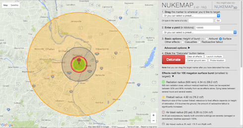
However, if we use the equation E = mc2, we can convert a 50 kg student into the explosive energy of the equivalent of 1,000,000 kilotons of TNT, which the newer website can’t quite handle.
Physics: Theories of Everything (Mapped)
An excellent overview of the multitude of active theories and hypotheses–like quantum gravity, string theory–physicists are investigating to try to explain the universe.
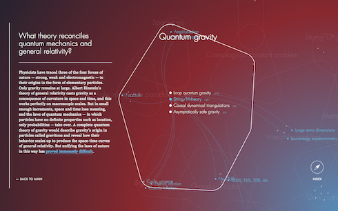
In the quest for a unified, coherent description of all of nature — a “theory of everything” — physicists have unearthed the taproots linking ever more disparate phenomena. With the law of universal gravitation, Isaac Newton wedded the fall of an apple to the orbits of the planets. Albert Einstein, in his theory of relativity, wove space and time into a single fabric, and showed how apples and planets fall along the fabric’s curves. And today, all known elementary particles plug neatly into a mathematical structure called the Standard Model. But our physical theories remain riddled with disunions, holes and inconsistencies. These are the deep questions that must be answered in pursuit of the theory of everything.
–Natalie Wolchover in Theories of Everything Mapped on Quanta Magazine.
Interactive Electric Fields (with Paper.js)
Drag the charges around.
The force field created by the interaction of two electric charges (one positive and one negative). The source is at http://soriki.com/fields/electric/.