Elon Musk would like to put his Tesla into Mars orbit. YouTube user ShadowZone shows how it could be done…using Kerbal Space Program. Awesome.
Tag: modeling
Modeling Earth’s Energy Balance (Zero-D) (Transient)
If the Earth behaved as a perfect black body and absorbed all incoming solar radiation (and radiated with 100% emissivity) the we calculated that the average surface temperature would be about 7 degrees Celsius above freezing (279 K). Keeping with this simplification we can think about how the Earth’s temperature could change with time if it was not at equilibrium.
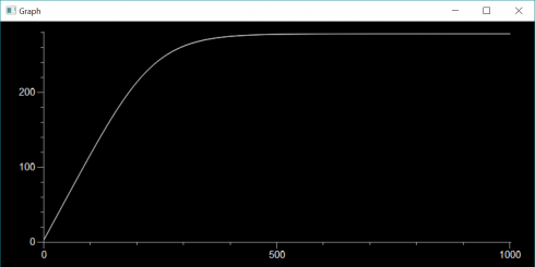
If the Earth started off at the universe’s background temperature of about 3K, how long would it take to get up to the equilibrium temperature?
Using the same equations for incoming solar radiation (Ein) and energy radiated from the Earth (Eout):


Symbols and constants are defined here except:
- rE = 6.371 x 10⁶ m
At equilibrium the energy in is equal to the energy out, but if the temperature is 3K instead of 279K the outgoing radiation is going to be a lot less than at equilibrium. This means that there will be more incoming energy than outgoing energy and that energy imbalance will raise the temperature of the Earth. The energy imbalance (ΔE) would be:

All these energies are in Watts, which as we’ll recall are equivalent to Joules/second. In order to change the temperature of the Earth, we’ll need to know the specific heat capacity (cE) of the planet (how much heat is required to raise the temperature by one Kelvin per unit mass) and the mass of the planet. We’ll approximate the entire planet’s heat capacity with that of one of the most common rocks, granite. The mass of the Earth (mE) we can get from NASA:
- cE = 800 J/kg/K
- mE = 5.9723×1024kg
So looking at the units we can figure out the the change in temperature (ΔT) is:

Where Δt is the time step we’re considering.
Now we can write a little program to model the change in temperature over time:
EnergyBalance.py
from visual import *
from visual.graph import *

I = 1367.
r_E = 6.371E6
c_E = 800.
m_E = 5.9723E24

sigma = 5.67E-8

T = 3                               # initial temperature

yr = 60*60*24*365.25
dt = yr * 100
end_time = yr * 1000000
nsteps = int(end_time/dt)

Tgraph = gcurve()

for i in range(nsteps):
    t = i*dt
    E_in = I * pi * r_E**2
    E_out = sigma * (T**4) * 4 * pi * r_E**2
    dE = E_in - E_out
    dT = dE * dt / (c_E * m_E)
    T += dT
    Tgraph.plot(pos=(t/yr/1000,T))
    if i%10 == 0:
        print t/yr, T
        rate(60)
The results of this simulation are shown at the top of this post.
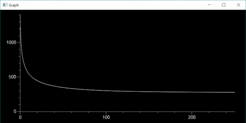
What if we changed the initial temperature from really cold to really hot? When the Earth formed from the accretionary disk of the solar nebula the surface was initially molten. Let’s assume the temperature was that of molten granite (about 1500K).
Modeling Earth’s Energy Balance (Zero-D) (Equilibrium)
Energy and matter can’t just disappear. Energy can change from one form to another. As a thrown ball moves upwards, its kinetic energy of motion is converted to potential energy due to gravity. So we can better understand systems by studying how energy (and matter) are conserved.
Energy Balance for the Earth
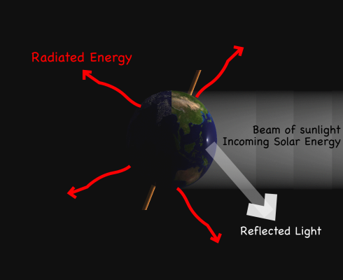
Let’s start by considering the Earth as a simple system, a sphere that takes energy in from the Sun and radiates energy off into space.
Incoming Energy
At the Earth’s distance from the Sun, the incoming radiation, called insolation, is 1367 W/m2. The total energy (wattage) that hits the Earth (Ein) is the insolation (I) times the area the solar radiation hits, which is the area a cross section of the Earth (Acx).

Given the Earth’s radius (rE) and the area of a circle, this becomes:
Outgoing Energy
The energy radiated from the Earth is can be calculated if we assume that the Earth is a perfect black body–a perfect absorber and radiatior of Energy (we’ve already been making this assumption with the incoming energy calculation). In this case the energy radiated from the planet (Eout) is proportional to the fourth power of the temperature (T) and the surface area that is radiated, which in this case is the total surface area of the Earth (Asurface):

The proportionality constant (σ) is: σ = 5.67 x 10⁻⁸ W m-2 K-4
Note that since σ has units of Kelvin then your temperature needs to be in Kelvin as well.
Putting in the area of a sphere we get:
Balancing Energy
Now, if the energy in balances with the energy out we are at equilibrium. So we put the equations together:


cancelling terms on both sides of the equation gives:

and solving for the temperature produces:

Plugging in the numbers gives an equilibrium temperature for the Earth as:
T = 278.6 K
Since the freezing point of water is 273K, this temperature is a bit cold (and we haven’t even considered the fact that the Earth reflects about 30% of the incoming solar radiation back into space). But that’s the topic of another post.
Modeling the Universe
A wonderful explanation of why scientists create computer models of the universe (and how it’s done); it’s a bit like the solar nebula model writ large.
(via The Dish).
Build Your Own Solar System: An Interactive Model
National Geographic has a cute little game that lets you create a two-dimensional solar system, with a sun and some planets, and then simulates the gravitational forces that make them orbit and collide with each other. The pictures are pretty, but I prefer the VPython model of the solar system forming from the nebula.
The models starts off with a cloud of interstellar bodies which are drawn together by gravitational attraction. Every time they collide they merge creating bigger and bigger bodies: the largest of which becomes the sun near the center of the simulation, while the smaller bodies orbit like the planets.
This model also comes out of Sherwood and Chabay’s Physics text, but I’ve adapted it to make it a little more interactives. You can tag along for a ride with one of the orbiting planets, which, since this is 3d, makes for an excellent perspective (see the video). You can also switch the trails on and off so you can see the paths of the planetary bodies, note their orbits and see the deviations from their ideal ellipses that result from the gravitational pull of the other planets.
I’ve found this model to be a great way to introduce topics like the formation of the solar system, gravity, and even climate history (the ice ages over the last 2 million years were largely impelled by changes in the ellipticity of the Earth’s orbit).
National Geographic’s Solar System Builder is here.