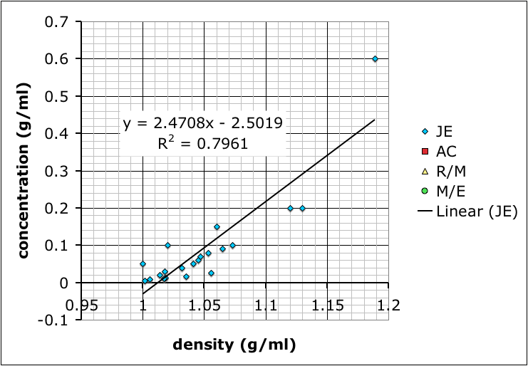
Calibration curves produced by different student groups to determine the relationship between density and concentration of salt (NaCl) solutions.
To start with chemistry class, we’re studying the properties of substances (like density) and how to measure and report concentrations. So, I mixed up four solutions of table salt (NaCl) dissolved in water of different concentrations, and put a drop of food coloring into each one to clearly distinguish them. The class as a whole had to determine the densities of the solutions, thus learning how to use the scales and graduated cylinders.
However, for the students interested in doing a little bit more, I asked them to figure out the actual concentrations of the solutions.
One group chose to evaporate the liquid and measure the resulting mass in the beakers. Others considered separating the salt electrochemically (I vetoed that one based on practicality.
Most groups ended up choosing to mix up their own sets of standard solutions, measure the densities of those, and then use that data to determine the densities of the unknown solutions. Their data is shown at the top of this post.
Finding the mass of solution in order to calculate its density.
The variability in their results is interesting. Most look like the result of systematic differences in making their measurements (different scales, different amounts of care etc.), but they all end up with curves where the concentration increases positively with density.
I showed the graph above to the class so we could talk about different sources of error, and how scientists will often compile the data from several different studies to get a better averaged result.
Then, I combined all the data and added a linear trend line so they could see how to do it using Excel (many of these students are in pre-calculus right now so it ties in nicely):
Trend line from combined data.
What we have not talked about yet–I hope to tomorrow–is how the R-squared value, which gives the goodness of the fit of the trend line to the data, is more a measure of precision rather than accuracy. It does say something about how internally consistent the data are, but not necessarily if the result is accurate.
It’s also useful to point out that the group with the best R-squared value is the one with only two data points because two data points will necessarily give a perfectly straight line. However, the groups that made more solutions might not have as good of an R-squared value, but, because of the multiple measurements, probably have more reliable results.
As for which group got the most accurate result: I added in some data I found by googling–it came off a UCSD website with no citation so I’m going to need to find a better reference. Comparing our data to the reference we find that team AC (the red squares) best match:
The straight line shows my (currently) accepted values for the concentration/density relationship.
Microsoft Excel, like most graphical calculators and spreadsheet programs, has the built in ability to do linear regression of measured data using certain types of functions — lines, polynomials, logarithms, and exponents for example. However, you can get it to do any type of function — sinusoidal, natural log, whatever — if you work through the spreadsheet and can use the iterative Solver tool.
This more general approach is quite useful in teaching pre-Calculus, because the primary purpose of all the functions they have to learn is to create mathematical models (functions) based on data that can be used for predictions.
The Data
I started this year’s pre-calculus class by having them collect some data. In a simplification of the snow-melt experiment I did with the middle school last year, I had them put a beaker of water (about 300ml) on a hot plate and measure the temperature every minute as warmed up.
To make the experiment a little more interesting, I had each student in each group of four take just three consecutive measurements and try to find the equation of the straight line that best fit their data, and could be used to try to predict the other measurements of their peers in their group.
Figure 1. Scatter plot of measured temperatures during the warming of a beaker of water on a hot plate. Data given in Table 1.
It did not quite work out as I’d hoped. Since you only need two points to find the equation of a straight line, having three points produced a little confusion. I’d hoped to produce that confusion, but hadn’t realized that I’d need to do a review of how to find the equation of a straight line. A large fraction of the class was a little bit rusty after hot months of summer.
So, we pooled all the data and reviewed how to find the equation of a straight line.
Table 1: The Data
Time (minutes)
Measured Temperature (°C)
0
22
1
26
2
31
3
36
4
40
5
44
6
48
7
53
8
58
9
61
10
65
11
68
12
71
Finding the Equation for a Straight Line using Two Points
The general equation for a straight lines is:
(1)
and we need to determine the coefficients m and b. m is the slope, which can be calculated from two points using the equation:
(2)
using the points at t=6 and t=11 — the points (x1, y1) = (6,48) and (x2, y2) = (11,68) respectively — for example, gives a slope of:
so our general equation becomes:
to find b we substitute either one of the points into the equation for x and y. If we use the first point, x = 6, and y = 48, we get:
and the equation of our line becomes:
(3)
Now, since we’re actually looking at a relationship between temperature and time, with temperature on the y-axis and time on the x-axis, we could relabel the terms in the equation with T = temperature and t = time to have:
(4)
While this equation is more satisfying to me, because I think it better describes the relationship we have, the more vocal students preferred the equation in terms of x and y (Eqn 3). These are the terms they are more familiar with in the context of a math class, and I recall seeing some evidence that students seem to learn better with the more abstract representations sometimes (though I can’t quite remember the source; I should have blogged about it).
Plotting the Data and the Modeled Straight Line
The straight line equation we came up with (Eqn. 4) is our model of the data. It’s not quite perfect. All the data do not lie on the line, although, if we did everything right, only the points (6, 48) and (11, 68) are guaranteed to be on the line.
Figure 2. The equation of our straight line model (red line) matches the data (blue diamonds) pretty well.
I showed the class how to plot the scatter graph using MS Excel, and how to draw the line to show the modeled data. The measured data are represented as points since the measurements were made at discrete points in time. The modeled equation, however, is a continuous function, hence the straight line. The Excel sheet below (Resource 1) illustrates:
The Excel spreadsheet (Resource 1) was set up so that when I entered the slope (m) and intercept (b) values, the graph would quickly update. So I went through the class. Everyone called out their slope and intercept values, I plugged them in, and they could all see how the modeled line changed slightly based on the points used to calculate it. So I put the question to them, “How can we figure out which model equation is the best?”
That’s how I was able to introduce the topic of error. What if we compared the temperature predicted by the model for each data point, to the actual value. The smaller the difference in modeled versus measured temperatures, the better the fit of the model. Indeed, if we sum all the differences, or better yet take the average of the differences, we could get a single number, we’ll call the average error (ε), that could be used to compare the different models. I used this opportunity to introduce sigma notation, which the pre-calculus students had not seen much of before.
As a first pass (which, as we’ll see below, has a major problem), the error (ε) for each point (i) is:
The average error is the sum of all the errors divided by the number of points (n) (we have 12 points so n=12 in this example):
(5)
Now this works, but there is one problem. I was quite pleased and a little bit surprise that one of my students recognized what it was without any coaxing and also suggested a solution: by simply taking the difference to calculate the error, a point that is offset above the modeled line can be canceled out by a point offset by the same amount below the line. So what we really need is to use the absolute value of the error.
(6)
This works, and is what we went with, but I did also point that what’s usually done is to use the square of the error instead of the absolute value. Squaring makes any number positive, so it accomplishes the same goal as the absolute value, and is the approach we’ll use when I go into linear regression later on.
Setting up the Excel spreadsheet to calculate the average error is fairly straightforward as shown in Resource 2:
So once again, we went through the class and everyone called out their slope and intercept values and cheered when I plugged the numbers in and they saw if they had the lowest value.
It is important to remember, though, that the competition gives a somewhat random result: students’ average error is a function of the points they happened to pick, not how well they did the math (assuming everyone did the math correctly).
Figure 2. Showing the spreadsheet used to calculate the average error (Resource 2).