A couple quick programs (polarGraphs.py) to create animations of the drawing of functions in polar coordinates (for my pre-Calculus class).
Graph of the function: r = 4 cos(θ)
It can export as a movie (mp4 as above). W can also transform functions (using: polarToCartesianGraph.py ) from rectangular to polar coordinates (and back: you can choose the settings).
Coordinate transforms Cartesian to Polar and back again for r = 4 cos(θ)
A Note on using ChatGPT
This python program uses the matplotlib library, and, for the first time for me, I used ChatGPT to figure out the syntax for things like drawing arcs and arrows, and exporting animation files, instead of googling my questions. ChatGPT worked great, and significantly speeded up the process. It does make me wonder, however, that since these models are based off of what they’ve scraped from the internet, are they going to run create problems for themselves if people stop asking questions on places like stackoverflow and rely on AI instead. Although, this might just mean that the AI will tend to be just be a little bit behind the cutting edge and there will continue to be a need for question and answer forums.
Teaching programming using the LED light strips is going much better than expected. I tried it with the 9th grade Algebra class during our weekly programming session using a set of coding lessons I put together. I went so well that though we started by having everyone (about 10 kids) share two LED strips, by the end of the year I had three students from that class build their own.
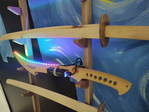
Student’s LED strip on a sword. The battery can power it for at least 15 minutes.
The coding lessons are still a work in progress, but it has them learn the basics by running some of the test programs, then then explore sequences using for loops. There are a lot of directions to branch off after the for loops. I’ve had some of my Algebra II students make static patterns using linear and exponential functions, while a couple of the kids in my programming class used different functions to make dynamic lighting patterns; our hydroponic system (see here and here) now has a neat LED indicator that runs different sequences depending on if the pumps are running or not.
Some of the students who built their LED strips in the Makerspace posted about their projects: LED Thingy and LED Light Strip Project. The process (rpi-led-strip) is not too hard but required them to be able to do a little physical computing (with Raspberry Pi’s), use ssh and terminal commands (terminal instructions), and then run and write python programs.
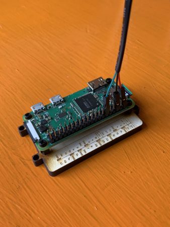
Raspberry Pi that controls one of the LED strips from a student’s project.
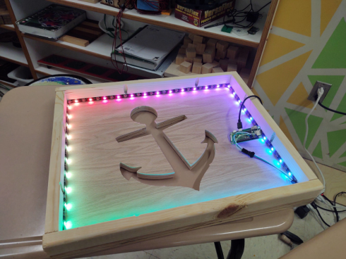
Since the setup uses the same GitHub repository (rpi-led-strip) it’s also easy to update some of our existing projects like the Wall Anchor.
Wall anchor project.
I am amazed at how much the students have engaged with what are, ultimately, very simple systems (a Raspberry Pi and a strip of 20 lights), and I’m really excited to see where it takes us.
In talking to alumni and their peers who have recently started computer science related careers, I have been encouraged to continue using python as the primary language for introducing students to programming.
I was recently pointed towards a very good Introduction to Python on the jobtensor website. It has a clean design and uses iPython Shells on the webpage so you can run some basic code on the site itself.
I’ve been using python as the primary programming language for all of my classes, from middle to high school. However, with a variety of different machines and operating systems–macs, PC’s, OSX, Windows, ChromeOS–it has been bit of a pain getting everyone up and running and on the same page. It has been especially problematic because I like to use NumPy and, especially, the VPython module because of its nice, easy 3d visualizations.
I’ve tried Anaconda, which works great on some machines but not so much on others. One student with a Mac had to restart the kernel every time he ran a program with vpython, while others had trouble getting it to work properly at all. I do like the way it allows you to put everything into a single Jupyter Notebook, which works nicely for teaching-length programming assignments, but becomes cumbersome for longer projects. Joel Grus goes into detail about why he does not like Notebooks for teaching; much of which I agree with. I do like the Spyder IDE a lot, but I’ve run into some computers that have problems with it (constant crashes).
So, I’ve been using Glowscript a lot with the lower grades. It’s online, so you only need a browser, and its made for vpython, so you can do a lot of the numerical work with it. However, because it’s online you can’t, understandably, get it to write output files to your computer–you have to copy and paste from its output. I’m also not sure how to import user-created modules, which further limits its utility for higher-level classes.
I’ve recently run into repl.it, and I’m having a student try it out in my Numerical Methods class. It looks quite promising as it seems to be able to manage files well and we’ve tried some basic numerical programs using numpy and matplotlib. However, I’ve not got it running vPython yet (although it’s come close).
(repl.it update): One of our other teachers has been trying repl.it with the middle school class and really likes it.
I’ve also recently discovered MakeCode. I’m looking into it for the lower grades, down to 6th grade or even earlier, because it lets you write programs for Minecraft, which is very popular with a remarkably broad age group. It lets you work in blocks, python, or JavaScript. From my poking around, the first couple of things it teaches you to do in Minecraft are write statements (to generate a chicken) and the loops (to generate a lot of chickens). I’ve asked one of my 9th grade, Minecraft players to investigate, so I should have some results to report soon.
At the moment, for my most advanced class, we’re taking a whatever-works approach. We’re learning about finite differences and using matplotlib to graph the output. I have one student, mentioned above, using repl.it, and another one using Jupyter Notebook on a Mac. A different Mac user is invoking IDLE from the command line because they prefer the IDLE IDE, but couldn’t get numpy to install properly with the python 3.9 version they’d installed earlier–the command-line IDLE actually goes to their Anaconda installation. I have one student, on a Windows machine, for whom everything just works and are using their regular IDLE installation. We spent the entire class period getting everyone up and running with something, but at least now everyone has at least one environment they can use. I’m curious to see what the kids who have multiple options are going to go with.
3d model of the Hawaiian island chain, rendered in OpenSCAD.
After a lot of hours of experimentation I’ve finally settled on a workable method for generating large-scale 3d terrain.
Data from the NGDC’s Grid Extraction tool. The ETOPO1 (bedrock) option gives topography and bathymetry. You can select a rectangle from a map, but it can’t be too big and, which is quite annoying, you can’t cross the antimeridian.
The ETOPO1 data is downloaded as a GeoTIFF, which can be easily converted to a png (I use ImageMagick convert).
The Hawaiian data with the downloaded grayscale.
Adjusting the color scale. One interesting property of the data is that it uses a grayscale to represent the elevations that tops out at white at sea-level, then switches to black and starts from there for land (see the above image). While this makes it easy to see the land in the image, it needs to be adjusted to get a good heightmap for the 3d model. So I wrote a python script that uses matplotlib to read in the png image as an array and then I modify the values. I use it to output two images: one of the topography and one of just land and water that I’ll use as a mask later on. Hawaiian Islands with adjusted topography and ocean-land.
The images I export using matplotlib as grayscale png’s, which can be opened in OpenSCAD using the surface command, and then saved as an stl file. Bigger image files are take longer. A 1000×1000 image will take a few minutes on my computer to save, however the stl file can be imported into 3d software to do with as you will.
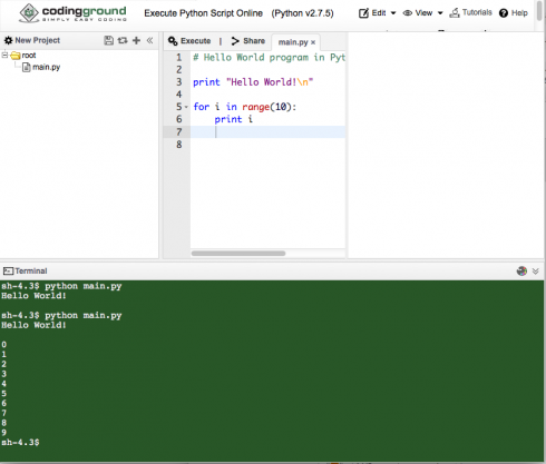
For some of my students with devices like Chromebooks, it has been a little challenging finding ways for them to do coding without a simple, built-in interpreter app. One interim option that I’ve found, and like quite a bit is the TutorialsPoint Coding Ground, which has online interfaces for quite a number of languages that are great for testing small programs, including Python.
Screen capture of Python coding at Tutorial Point’s Coding Ground.
Working on algebra over the summer, we tried a little programming. This is O’s first program, which gives the chirp rate of crickets based on the temperature.
t = float(raw_input('enter temperature> '))

n=4*t-160
print "number of chirps=", n
print "t=", t
Numerical integration is usually used for functions that can’t be integrated (or not easily integrated) but for this example we’ll use a simple parabolic function so we can compare the numerical results to the analytical solution (as seen here).
With the equation:
To find the area under the curve between x = 1 and x = 5 we’d find the definite integral:
For numerical integration, we break the area of concern into a number of trapezoids, find the areas of all the trapezoids and add them up.
We’ll define the left and right boundaries of the area as a and b, and we can write the integral as:
The left and right boundaries of the area we’re interested in are defined as a and b respectively. The area of each trapezoid is defined as An.
We also have to choose a number of trapezoids (n) or the width of each trapezoid (dx). Here we choose four trapezoids (n = 4), which gives a trapezoid width of one (dx = 1).
The area of the first trapezoid can be calculated from its width (dx) and the height of the two upper ends of the trapezoid (f(x0) and f(x1).
So if we define the x values of the left and right sides of the first trapezoids as x0 and x1, the area of the first trapezoid is:
For this program, we’ll set the trapezoid width (dx) and then calculate the number of trapezoids (n) based on the width and the locations of the end boundaries a and b. So:
and the sum of all the areas will be:
We can also figure out that since the x values change by the same value (dx) for every trapezoid, it’s an arithmetic progression, so:
and,
so our summation becomes:
Which we can program with:
numerical_integration.py
# the function to be integrated
def func(x):
    return -0.25*x**2 + x + 4

# define variables
a = 1.          # left boundary of area
b = 5.          # right boundary of area
dx = 1          # width of the trapezoids

# calculate the number of trapezoids
n = int((b - a) / dx)

# define the variable for area
Area = 0

# loop to calculate the area of each trapezoid and sum.
for i in range(1, n+1):
    #the x locations of the left and right side of each trapezpoid
    x0 = a+(i-1)*dx
    x1 = a+i*dx

    #the area of each trapezoid
    Ai = dx * (func(x0) + func(x1))/ 2.

    # cumulatively sum the areas
    Area = Area + Ai

#print out the result.
print "Area = ", Area
And the output looks like
>>>
Area =  17.5
>>>
While the programming is pretty straightforward, it was a bit of a pain getting Python to work for one of my students who is running Windows 8. I still have not figured out a way to get it to work properly, so I’m considering trying to do it using Javascript.
Update
The javascript functions for numerical integration:
function numerically_integrate(a, b, dx, f) {

	// calculate the number of trapezoids
	n = (b - a) / dx;

	// define the variable for area
	Area = 0;

	//loop to calculate the area of each trapezoid and sum.
	for (i = 1; i <= n; i++) {
		//the x locations of the left and right side of each trapezpoid
		x0 = a + (i-1)*dx;
		x1 = a + i*dx;

		// the area of each trapezoid
		Ai = dx * (f(x0) + f(x1))/ 2.;

		// cumulatively sum the areas
		Area = Area + Ai

	}
	return Area;
}

//define function to be integrated
function f(x){
	return -0.25*Math.pow(x,2) + x + 4;
}

// define variables
a = 1;		// left boundary of area
b = 5;		// right boundary of area
dx = 1;		// width of the trapezoids

// print out output
alert("Area = "+ numerically_integrate(a, b, dx, f));
I’ve added the above javascript code to the embeddable graphs to allow it to calculate and display numerical integrals: you can change the values in the interactive graph below.