A Visual Introduction to Differentiation (using vpython)

Screen capture: Enter an x value and the program calculates the slope for the function and draws the tangent line.

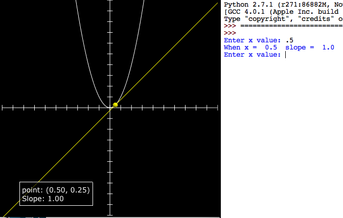
This quick program is intended to introduce differentiation as a way of finding the slope of a line. Students know how to find the slope of a tangent line at least conceptually (by drawing). We pick a curve: in this case:

 f(x) = x^2

then enter values of x in the program to see how x, the function value and the differential compare to each other.

x f(x) f'(x)
0.5 0.25 1
1 1 2
2 2 4
3 9 6

Because it’s quick you have to change the function in the code, and enter the values for x in the python shell.

With a sin curve.
With a sin curve.

differentiation_intro_numeric.py

from visual import *

class tangent_line:
    def __init__(self):
        self.dx = 0.1
        self.line = curve()
        self.tangent_line = curve()
        self.point = sphere(radius=.25,color=color.yellow)
        self.point.visible = False
        self.label = label(pos=(-5,-8))

    '''CHANGE FUNCTION (y) HERE'''
    # the original function
    def f(self, x):
        #y = sin(x)
        y = x**2
        return y
    '''END CHANGE FUNCTION HERE'''

    def find_slope(self, x):
        sdx = .00001
        m = (self.f(x+sdx)-self.f(x))/sdx
        return round(m,3)
        
    def draw(self):
        for x in arange(xmin, xmax+self.dx, self.dx):
            self.line.append(pos=(x, self.f(x)))

    def draw_tangent(self, x):
        m = self.find_slope(x)
        y = self.f(x)
        b = y - m * x
        print "When x = ", x, " slope = ", m
        self.label.text = "point: (%1.2f, %1.2f)\nSlope: %1.2f" % (x,y,m)
        self.plot_point(x)

        #draw tangent
        self.tangent_line.visible = False
        self.tangent_line = curve(pos=[(xmin,m*xmin+b),(xmax,m*xmax+b)], color=color.yellow)
              
    def plot_point(self, x):
        self.point.visible = True
        self.point.pos = (x, self.f(x)) 

#axes
xmin = -10.
xmax = 10.
ymin = -10.
ymax = 10.
xaxis = curve(pos=[(xmin,0),(xmax,0)])
yaxis = curve(pos=[(0,ymin),(0,ymax)])

#tick marks
tic_dx = 1.0
tic_h = .5
for i in arange(xmin,xmax+tic_dx,tic_dx):
    tic = curve(pos=[(i,-0.5*tic_h),(i,0.5*tic_h)])
for i in arange(ymin,ymax+tic_dx,tic_dx):
    tic = curve(pos=[(-0.5*tic_h,i),(0.5*tic_h,i)])

#stop scene from zooming out too far when the curve is drawn
scene.autoscale = False

# draw curve
func = tangent_line()
func.draw()

# get input
while 1:
    xin = raw_input("Enter x value: ")
    func.draw_tangent(float(xin))


Slope Fields

[inline]

Your browser does not support the canvas element.

[script type=”text/javascript”]
var width=500;
var height=500;
var xrange=10;
var yrange=10;

mx = width/(2.0*xrange);
bx = width/2.0;
my = -height/(2.0*yrange);
by = height/2.0;

function draw9083(ctx, polys) {
t=t+dt;
//ctx.fillText (“t=”+t, xp(5), yp(5));
ctx.clearRect(0,0,width,height);

polys[0].drawAxes(ctx);
polys[0].slopeField(ctx, 1.0, 1.0, 0.5);
ctx.lineWidth=2;
polys[0].draw(ctx);
polys[0].write_eqn(ctx, “dy/dx “);

}

//init_mouse();

var c9083=document.getElementById(“myCanvas9083”);
var ctx9083=c9083.getContext(“2d”);

var change = 0.0001;

function create_lines9083 () {
//draw line
//document.write(“hello world! “);
var polys = [];
polys.push(addPoly(0, 0.5, 1));

return polys;
}

var polys9083 = create_lines9083();

var x1=xp(-10);
var y1=yp(1);
var x2=xp(10);
var y2=yp(1);
var dy=0.01;

var t = 0;
var dt = 50;
end_ct = 0;

var move_dir = 1; // 1 for up

//draw9083();
//document.write(“x”+x2+”x”);
//ctx9083.fillText (“n=”, xp(5), yp(5));
setInterval(“draw9083(ctx9083, polys9083)”, dt);

[/script]
[/inline]

Say you have the equation that gives you the slope of a curve (let  \frac{dy}{dx} ) be the slope):
! \frac{dy}{dx} = \frac{1}{2} x + 1

When you use integration to solve the equation, there are quite the number of possible solutions (infinite actually), because when you integrate:

! y = \int (\frac{1}{2} x + 1 ) dx

you get:
! y = \frac{1}{4} x^2 + x + c

where c is a constant. Unfortunately, you don’t know what c is without more information; it could be anything.

However, even without integrating, we can get a feel for what the curve will look like by plotting what the slope will look like at a bunch of different points in space. This comes in really handy when you end up with a equation for slope that is really hard — or even impossible — to solve.

The graph below show a curve of possible solutions to the slope equation. You should be able to see, as the graph slowly moves up and down, how the slope of the graph corresponds to the slope field.

[inline]

Your browser does not support the canvas element.

[script type=”text/javascript”]
var width=500;
var height=500;
var xrange=10;
var yrange=10;

mx = width/(2.0*xrange);
bx = width/2.0;
my = -height/(2.0*yrange);
by = height/2.0;

function draw9083b(ctx, polys) {
t9083b=t9083b+dt9083b;
//ctx.fillText (“t=”+t, xp(5), yp(5));
ctx.clearRect(0,0,width,height);

polys[0].drawAxes(ctx);
polys[0].slopeField(ctx, 1.0, 1.0, 0.5);
ctx.lineWidth=2;
polys[0].draw(ctx);
polys[0].write_eqn(ctx, “dy/dx “);

if (polys[1].c > yrange) {
move_dir9083b = -1.0;
polys[1].c = yrange;
}
else if (polys[1].c < -yrange) { move_dir9083b = 1.0; polys[1].c = -yrange; } polys[1].c = polys[1].c + dc9083b*move_dir9083b; polys[1].draw(ctx); polys[1].write_eqn(ctx); //ctx.fillText (' c='+move_dir9083b+' '+polys[1].c, xp(5), yp(5)); } //init_mouse(); var c9083b=document.getElementById("myCanvas9083b"); var ctx9083b=c9083b.getContext("2d"); var change = 0.0001; function create_lines9083b () { //draw line //document.write("hello world! "); var polys = []; polys.push(addPoly(0, 0.5, 1)); polys.push(addPoly(0.25, 1, 0)); polys[1].color = '#8C8'; return polys; } var polys9083b = create_lines9083b(); var x1=xp(-10); var y1=yp(1); var x2=xp(10); var y2=yp(1); var dc9083b=0.05; var t9083b = 0; var dt9083b = 100; //end_ct = 0; var move_dir9083b = 1.0; // 1 for up //draw9083b(); //document.write("x"+x2+"x"); //ctx9083b.fillText ("n=", xp(5), yp(5)); setInterval("draw9083b(ctx9083b, polys9083b)", dt9083b); [/script] [/inline]