2012 – Page 14 – Montessori Muddle

Switch: Converting Audio Files for Sound Effects

Adding sound to webpages is pretty easy with HTML5’s Audio tag (as Jean-Baptiste Jung demonstrates), but since different browsers can only handle certain, different types of sound files, you’ll often need to convert your sound into .wav, .ogg, and .mp3 formats so they can work for everyone.

Switch Sound File Converter does just what it says, and is free for non-commercial use.

ZygoteBody: Human Anatomy in 3D

With a simple, but effective interface, ZygoteBODY’s free, online 3d models of human anatomy are excellent.

zygote_body-anatomy-150c — Screen captures of ZygoteBODY's 3d model of the human digestive system.

Anatronica: 3d Anatomy Online

anatronica-3d-200 — Screen captures from Anatronica's Anatomy 3D Systems website. The digestive system is highlighted, while the skeletal system is shown semi-transparently for context.

Anatronica has an excellent, online, 3d viewer for the anatomy of the human torso. While it’s not quite the same as a physical model, it’s pretty good as a study guide for middle schoolers.

Endothermic Reactions: Vinegar and Baking Soda

A quick and simple experiment that demonstrates endothermic reaction and can include a discussion of ionic and covalent bonds. Mixing baking soda and vinegar together drops the temperature of the liquid by about 4 °C in one minute. (Note that while the temperature drops and the reaction looks endothermic, it’s actually not — other things cause the cooling. However, since it looks like an endothermic reaction I use it as a first approximation of one.)

Ingredients

3 g baking soda – (sodium bicarbonate – NaHCO₃)
60 ml vinegar – (acetic acid – CH₃COOH)
200 ml styrofoam cup (needs to be big enough to contain the bubbles).
thermometer

Procedure

Add the baking soda to the vinegar in the styrofoam cup. Measure the temperature while stirring for about a minute.

Results

Time (t)	Temperature (°C)
0	25
15	24
30	21
60	21

Discussion

The chemical reaction between baking soda (sodium bicarbonate) and vinegar (acetic acid) can be written:

NaHCO₃ + CH₃COOH —-> CO₂ + H₂O + CH₃OONa

The products of the reaction are carbon dioxide gas (which gives the bubbles), water, and sodium acetate.

However, a more detailed look shows that for the reaction to work the two chemicals need to be dissolved in water. Dissolving these ionic compounds causes the two ions to separate. Dissolved baking soda dissociates into a sodium and a bicarbonate ion:

sodium bicarbonate —-> sodium ion + bicarbonate ion

NaHCO₃ —-> Na⁺ + HCO₃^–

Why doesn’t the bicarbonate break into smaller pieces? Because it’s atoms are bonded together more tightly by covalent bonds.

Similarly, the acetic acid in vinegar dissociates into:

acetic acid —-> hydrogen ion + acetate

CH₃COOH —-> H⁺ + CH₃COO^–

This video has a nice overview of ionic versus covalent bonding.

References

More detail about the reaction can be found at:

Wayne (accessed 2012): Baking Soda and Vinegar Reaction and Demonstrations, on http://apple-cider-vinegar-benefits.com

Exponential Cell Growth

The video shows 300 seconds of purely exponential growth (uninhibited), captured from the exponential growth VAMP scenario. Like the exponential growth function itself, the video starts off slowly then gets a lot more exciting (for a given value of exciting).

The modeled growth is based on the exponential growth function:

$N = N_0 e^{rt}$ (1)

where:

N = number of cells (or concentration of biomass);
N₀ = the starting number of cells;
r = the rate constant, which determines how fast growth occurs; and
t = time.

Finding the Rate Constant/Doubling Time (r)

You can enter either the rate constant (r) or the doubling time of the particular organism into the model. Determining the doubling time from the exponential growth equation is a nice exercise for pre-calculus students.

Let’s call the doubling time, t_d. When the organism doubles from it’s initial concentration the growth equation becomes:

$2N_0 = N_0 e^{r t_d}$

divide through by N₀:

$2 = e^{r t_d}$

take the natural logs of both sides:

$\ln 2 = \ln (e^{r t_d})$

bring the exponent down (that’s one of the rules of logarithms);

$\ln 2 = r t_d \ln (e)$

remember that ln(e) = 1:

$\ln 2 = r t_d$

and solve for the doubling time:

$\frac{\ln 2}{r} = t_d$

Decay

A nice follow up would be to solve for the half life given the exponential decay function, which differs from the exponential growth function only by the negative in the exponent:

$N = N_0 e^{-rt}$

The UCSD math website has more details about Exponential Growth and Decay.

Finding the Growth Rate

A useful calculus assignment would be to determine the growth rate at any point in time, because that’s what the model actually uses to calculate the growth in cells from timestep to timestep.

The growth rate would be the change in the number of cells with time:

$\frac{dN}{dt}$

starting with the exponential growth equation:

$N = N_0 e^{rt}$

since we have a natural exponent term, we’ll use the rule for differentiating natural exponents:

$\frac{d}{dx}(e^u) = e^u \frac{du}{dx}$

So to make this work we’ll have to define:

$u = rt$

which can be differentiated to give:

$\frac{du}{dt} = r$

and since N₀ is a constant:

$N = N_0 e^{u}$

$\frac{dN}{dt} = N_0 e^{u} \frac{du}{dt}$

substituting in for u and du/dt gives:

$\frac{dN}{dt} = N_0 e^{rt} (r)$

rearranging (to make it look prettier (and clearer)):

$\frac{dN}{dt} = N_0 r e^{rt}$ (2)

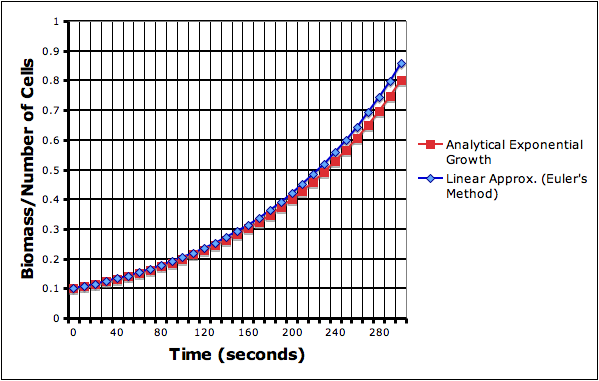
Numerical Methods: Euler’s method

With this formula, the model could use linear approximations — like in Euler’s method — to simulate the growth of the biomass.

First we can discretize the differential so that the change in N and the change in time (t$) take on discrete values:
$\frac{dN}{dt} = \frac{\Delta N}{\Delta t}$

Now the change in N is the difference between the current value N^t and the new value N^t+1:

Now using this in our differentiated equation (Eq. 2) gives:

$\frac{N^{t+1}-N^t}{\Delta t} = N_0 r e^{r\Delta t}$

Which we can solve for the new biomass (N^^t+1):

$N^{t+1}-N^t = N_0 r e^{r\Delta t} \Delta t$

to get:
$N^{t+1} = N_0 r e^{r\Delta t} \Delta t + N^t$

This linear approximation, however, does introduce some error.

The approximated exponential growth curve (blue line) deviates from the analytical equation. The deviation compounds itself, getting worse exponentially, as time goes on.

Excel file for graphed data: exponential_growth.xls

VAMP

This is the first, basic but useful product of my summer work on the IMPS website, which is centered on the VAMP biochemical model. The VAMP model is, as of this moment, still in it’s alpha stage of development — it’s not terribly user-friendly and is fairly limited in scope — but is improving rapidly.

Scale of the Universe

Another, excellent example showing the scale of the universe (only goes the size of the hydrogen atom though: this one goes a bit deeper).

The Universe made possible by Number Sleuth