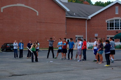
The middle school has been studying The Tempest over the last quarter. In order to give students a deeper connection with this Shakespearean play, we arranged for students to experience the titular meteorological phenomenon on our outdoor education trip last week. Since we’re located in the mid-continent, replicating the precise maritime conditions and acquiring the appropriate vessel would have been cost prohibitive. Instead, taking advantage of the local geography and socio-cultural predilections, we improvised by arranging for a series of thunderstorms during a canoe trip in the Ozarks.
In truth, the main purpose of our outdoor education trip was to integrate the upcoming 7th graders and new students into the middle school class. The key advantage of the multi-aged classroom is the opportunity for older students to mentor the younger students, and propagate the appropriate classroom culture and expectations from year to year. But for this to work well requires students to develop strong working relationships and communication skills. The isolation of the trip (no technology) and the coordination required for the tasks we perform (such as paddling a 2-person canoe) greatly facilitate this process.
Despite being drenched, chilled, and a little scared, the group’s performance was remarkable. They endured the worst of the storms, looking out for each other with encouraging words and heartening smiles. They found the strength within themselves as individuals and as a group to keep morale high while on the river. And, when we pulled over, were able to bask in the giddy relief that a good group feels after stressful situations. By the end, they had developed a genuine camaraderie forged by a shared, intense challenge.
P.S. We also did some rock climbing, caving, spent a night on a sandbar, journaled, and learned a bit about geology, hydrogeology, fish surveys, the rock cycle, and some vocabulary (“hubris” was a term, new to many, that was ably demonstrated by the pair who flipped their canoe).
P.P.S. Our excellent, invaluable guides on the trip were from Discovery Ministries, which is a religious organization, but they do non-religious programs for groups like ours.
The middle school class has been reading The Tempest for language arts this semester. However, I had not quite realized that it was a presentiment of for our outdoor education canoeing trip. And not metaphorically — the group worked amazingly well together — but there really was a massive storm while we were out paddling on the Current River.
On Wednesday morning, two hours before dawn, a cold front heading south from Canada met a warm front coming north out of the Gulf. They met and stalled, pushing waves of clouds and thunderstorms over us from the west.
The first wave hit while we were in our tents; the second during breakfast. One student recounted that his highest point of the trip was when he tasted his first pancake that morning. His lowest point was when the pancake was promptly soaked with rain.
The third wave met us while we were in our canoes.
Searing lightning, flashing across the ridges of the valley. Blinding white. Immediate thunder, roaring straight through the ears, reaching in, taking the breath, grabbing at the soul. Drenching rain — cold and hard — a deluge. One of our guides described it, afterwards, as a religious experience. I think I know what she meant.
But the kids were awesome. Drenched, cold, and scared they paddled on. I was with a small group that was bringing up the rear. We were far enough behind that, for a long time, I could not tell how the students in the lead were responding. Especially when, at the height of the downpour, the lead group went around a bend in the river and out of our line of sight.
I knew they were with our lead guide (Leah), whose skill and competence had already been demonstrated earlier in the day when one of the canoes had flipped. Yet, one always worries about how kids will react in stressful situations. Following the current around a gravel eyot, however, I heard a loud cheer. There was the line of canoes, pulled over waiting for us. There were the students, soaked and perhaps a little bit relieved, but with no panic in the cacophony of voices.
When everyone had caught up, we continued on. Eventually, we hit a landing and called an end to the canoeing. Although the rain had stopped it was still cold. So, a few students decided that since the river water was so cold, if they waited in the water, when they came out they’d feel warm. “I’m willing to deceive my body,” they said.
While we waited for the bus, we talked a little about what we’d been through. Despite the stress — or perhaps because of — there was lots of laughter and a growing sense of camaraderie. I took the chance to highlight some of the quieter voices, those students who tend not to complain or be too excitable, and who took the time to appreciate the beauty and uniqueness of what they’d been through.
While I would not have planned it that way, the storm, our tempest, forged bonds of common experience that will resonate with this group for years to come.
Notes
Infra-red satellite imagery from Wednesday, September 26th, 2012 shows the waves of thunderstorms passing over southern Missouri (yellow dot) very well.
If children live with criticism, they learn to condemn.
If children live with hostility, they learn to fight.
If children live with fear, they learn to be apprehensive.
If children live with pity, they learn to feel sorry for themselves.
If children live with ridicule, they learn to feel shy.
…
If children live with encouragement, they learn confidence.
…
If children live with acceptance, they learn to love.
…
If children live with sharing, they learn generosity.
If children live with honesty, they learn truthfulness.
If children live with fairness, they learn justice.
If children live with kindness and consideration, they learn respect.
If children live with security, they learn to have faith in themselves and in those about them.
C.G.P.Grey lays out the problems with the U.S.A’s current “first past the post/winner take all” voting system and then explains how to fix them:
The problems:
Minority rule: You can win with less than half the vote (at least in the beginning).
Inevitable, unavoidable, two-party system evolves over time.
Third-parties become spoilers; the better a third-party does the worse it is for their voters because it takes away votes from the other party they would favor.
Here I’ll go over how to do Least Squares Regression, as simply as possibly, using Excel and its Solver*. Least Squares Regression can be used to match pretty much any type of function to any type of data. Most spreadsheet programs, like Excel, will do some curve matching for you when you add trendlines to graphs, but for more sophisticated work — in pre-Calculus and beyond for example — you need a more general approach.
We’ll start with a data set that we want to match. The atmospheric CO2 data from Mauna Loa is a convenient dataset. It’s also an important data set to model because matching a function to the data will allow us to predict the change in CO2 over the next 100 years, and those predictions are the ones the IPCC uses in their estimates of the impact of global climate change around the world. Billions, if not trillions of dollars depend on those predictions (and how governments decide to respond). For ease of demonstration, I’ve picked a few of the annual average CO2 concentration measurements at random to work with:
Table 1: CO2 Data
Year (x)
CO2 concentration (ppm) (y)
1959
315.97
1964
319.62
1969
324.62
1981
340.10
1985
346.04
1996
362.59
2003
375.77
Now, looking at the data, we can see there is some sort of trend. Our first decision is about how to model it.
Straight Line Model
The simplest approach, and the one we’ll try first is to fit a straight line through the data. (The final spreadsheet is here).
The equation of a straight line is:
In this case, as we can see from the graph (Figure 1), the y axis is CO2 concentration, and the x axis is the year. m and b are our two unknown constants that set the slope of the line (m) and move it up and down (b). If you need to get a better feel for what this means, try changing the slope and intercept in the Straight Line Grapher (I used this in class to demonstrate).
To match our straight line model to the data we need to determine the values of m and b that give the best fit.
So we create a spreadsheet with the data and in the adjacent column set up the straight line function by setting two cells to the values of the constants (m and b) and using those values to calculate the modeled CO2 concentration.
You’ll notice that I have values of m = 1 and b = -1600 . These are just my initial estimates of these values. The initial values are not crucial, as you’ll see, but are just there for me to check that my formula is in right.
Once I have the correct formulas in, I can play around with these values until my line matches the data. However, this is where Solver comes in to save a lot of time.
Finding a match
First we need a quantitative way of telling if we have a good match or not. We can start by taking the difference between each real data point and the modeled value. We’ll call this the error.
Now we could get a single value for the total error by adding up all the individual error values, or taking the average. However, as one of my students pointed out, we could end up with a case where the modeled line crossed through the data and we’d end up with positive differences of the data points above the line canceling out the negative differences of the data points below the line. His solution was to take the absolute value of the differences (errors) instead, which should actually work just as well in the method we’re taking here.
Instead of using the absolute value, however, we’ll square the errors instead. This achieves the same effect we need because the squares of both negative and positive numbers are positive. This approach is where the “squares” in Least Squares Regression comes from. The “Least” part comes from the fact that we’re now going to try adjusting our coefficients until we get the average of the squares of the errors to be as small as possible.
Now we take the calculate the average of the errors (the sum of the errors would work just as well) using the spreadsheet’s “AVERAGE” function.
Now we can adjust m and b and not just see how they compare to the data points on a graph, but know that we have the best fit if we minimize the average error.
Solver
Instead of changing m and b by hand, we can use Excel’s Solver to minimize the average error for us. The matching of a straight line can be done using algebra (e.g. here and here) but that approach won’t help us when we get to more complex functions.
We select the average error cell (E16) and tell Solver to minimize its value by changing the values of m and b.
When we hit solve, Solver should converge on a solution. Because of the way the problem is set up — using the square of the error for example — makes this a non-linear problem for the solver to solve. As of this writing, Excel is the only spreadsheet program I know of that has a built-in, non-linear solver.
You’ll notice that Solver’s solution gives:
m = 1.360
b = -2351.9
So now we have the equation for the best fit line (our model) being:
Prediction
Using this model we can predict the atmospheric CO2 concentration for the year 2050 by setting x = 2050 in the modeled equation, which gives 436.5 ppm.
The final spreadsheet I used to do these calculations can be found here.
Parabolic Model
As good as the straight line model seems to be, it does not account for the slight upward curve the data seems to have (see Figure 1). So instead of a straight line, perhaps we could try a parabolic function. Just as before, we’ll need to figure out the coefficients for the parabolic function. In this case the general equation we’ll use is:
and we’ll need to find the coefficients a, b and c. To see how changing these coefficients change the curve, you can play around with the interactive parabola model.
We set up our spreadsheet in the same way as for the straight line, but with our new coefficients.
Note that the only column that needs to change from the straight-line spreadsheet is the “Model” column (column C), to add the coefficients and to change the formula to that of a parabola.
Now we can use Solver to minimize the average of the squares of the errors, just as we did before, only having it change the three coefficients instead of two.
a = 0.00060091
b = -1.018
c = 0.9933
and a final equation:
Prediction
The parabolic model predicts for the year 2050 (x = 2050) that the CO2 concentration will be 439.4 ppm.
The Excel spreadsheet for the parabolic model is here.
Which model is better?
The easiest way to compare the two models is to see which did better at minimizing the squared errors.
Table 2: Comparison of models.
Model
Average Squared Error
Straight Line
4.94
Parabola
4.47
So the parabolic model does better, but not by much.
Conclusions
With this approach, you can use any type of function — exponential, sinusoidal etc. — or combination of functions to match any data, and be able to compare among the models. A better measure of how well the models match the data is the regression coefficient or coefficient of determination, but I’ll save those for another post.
Conclusions
* UPDATE (Dec 31, 2012): Gnumeric’s Solver works.
* You’ll need to use Microsoft’s Excel, or better yet Gnumeric for this because, as of this writing, none of the other common spreadsheet options — OpenOffice, Google Docs, and Mac’s Calc — have a non-linear solver built in — and even some of the newer versions of Excel seem buggy.
Perhaps the key reason for the profound influence of Darwin’s “On the Origin of Species” is that it’s such a well written and well reasoned argument based on years of study. It is a wonderful example of how science should be done, and how it should be presented. In the past I’ve had my middle schoolers try to translate sections of Darwin’s writing into plainer, more modern English, with some very good results. They pick up a lot of vocabulary, and are introduced to longer, more complex sentences that are, however, clearly written.
The text of “On the Origin of Species” is available for free from the Gutenberg library. Images of the original document can be found (also for free) at the UK website, Darwin Online (which also includes the Darwin’s annotated copy). Darwin Online also hosts lot of Darwin’s other works, as well as notes of the other scientists on The Beagle, among which is included some wonderful scientific diagrams.
This year, I’m going to have the middle schoolers read the introduction, while the honors environmental science students will read selected chapters and present to the class — this will be their off-block assignment.