What is Real? A Math Seminar (Prelude to Imaginary Numbers)

We had a really nice, thoughtful seminar discussion in Algebra II, with the simple question: What is real?

I did this as a lead into the topic of imaginary numbers (i = \sqrt{-1}).

The distinction between tangible and intangible objects came up pretty early in the discussion. That morphed pretty quickly with the realization that there were things that you can’t touch, like ideas and thoughts that were real as well, despite being non-physical.

Then they considered some of the more edge-wise cases, such as, are dragons real. After all, they never really existed, but are parts or real myths. That thought lead to the idea that anything that was thinkable–anything you could think of–was real.

I jumped in, near the end, to insert the idea that maybe there were things that were not real–that were imaginary–but could be useful. And that’s how I set up my lesson on imaginary numbers.

Because even if you can’t calculate the square root of -1 (no number times itself will give a negative number).

 \sqrt{-1} = ?

You can give it a name.

 i = \sqrt{-1}

And under certain circumstances:

 i \cdot i = i^2

You might find that imaginary numbers can combine to give you real numbers.

 i^2 = (\sqrt{-1} )^2

 i^2 = -1

Which means we can do a whole lot of calculations that were impossible before, making imaginary numbers extremely useful.

 \sqrt{-9} \cdot \sqrt{-4} = 3i \cdot 2i  = 6 \cdot i^2 = 6 \cdot (-1) = -6

Dilation

Dilation (scaling) of a quadrilateral by 2x.

A quick program that animates scaling (dilation) of shapes by scaling the coordinates. You type in the dilation factor.

dilation.py

from visual import *

#axes
xmin = -10.
xmax = 10.
ymin = -10.
ymax = 10.
xaxis = curve(pos=[(xmin,0),(xmax,0)])
yaxis = curve(pos=[(0,ymin),(0,ymax)])

#tick marks
tic_dx = 1.0
tic_h = .5
for i in arange(xmin,xmax+tic_dx,tic_dx):
    tic = curve(pos=[(i,-0.5*tic_h),(i,0.5*tic_h)])
for i in arange(ymin,ymax+tic_dx,tic_dx):
    tic = curve(pos=[(-0.5*tic_h,i),(0.5*tic_h,i)])

#stop scene from zooming out too far when the curve is drawn
scene.autoscale = False

# define curve here
shape = curve(pos=[(-1,2), (5,3), (4,-1), (-1,-1)])

shape.append(pos=shape.pos[0])
shape.color = color.yellow
shape.radius = 0.1
shape.visible = True

#dilated shape
dshape = curve(color=color.green, radius=shape.radius*0.9)
for i in shape.pos:
    dshape.append(pos=i)

#label
note = label(pos=(5,-8),text="Dilation: 1.0", box=False)
intext = label(pos=(5,-9),text="> x", box=False)

#scaling lines
l_scaling = False
slines = []
for i in range(len(shape.pos)):
    slines.append(curve(radius=shape.radius*.5,color=color.red, pos=[shape.pos[i],shape.pos[i],shape.pos[i]]))


#animation parameters
animation_time = 1. #seconds
animation_smootheness = 30
animation_rate = animation_smootheness / animation_time

x = ""
while 1:
    #x = raw_input("Enter Dilation: ")
    if scene.kb.keys: # event waiting to be processed?
        s = scene.kb.getkey() # get keyboard info

        #print s
        if s <> '\n':
            x += s
            intext.text = "> x "+x
        else:
            try:
                xfloat = float(x)
                note.text = "Dilation: " + x

                endpoints = []
                dp = []
                for i in shape.pos:
                    endpoints.append(float(x) * i)
                    dp.append((endpoints[-1]-i)/animation_smootheness)
                #print "endpoints: ", endpoints
                #print "dp:        ", dp
                for i in range(animation_smootheness):
                    for j in range(len(dshape.pos)):
                        dshape.pos[j] = i*dp[j]+shape.pos[j]
                    rate(animation_smootheness)
                    if slines:
                        for i in range(len(shape.pos)):
                            slines[i].pos[1] = vector(0,0)
                            slines[i].pos[-1] = dshape.pos[i]

                for i in range(len(shape.pos)):
                    dshape.pos[i] = endpoints[i]
                    slines[i].pos[-1] = dshape.pos[i]

                for i in range(len(shape.pos)-1):
                    print shape.pos[i], "--->", dshape.pos[i]
                    
            except:
                #print "FAIL"
                failed = True
                intext.text = "> x "
            x = ""


Transformations and 3D Printing

My pre-algebra class is working on transformations, so it seemed a good opportunity to try some 3d printing. I showed them how to create basic shapes (sphere, triangle, and box) and how to move them (transform) in a three-dimensional coordinate system using OpenScad.

Students create their car models using OpenScad.

Then we started printing them out on our 3d printer. Since it takes about an hour to print each model, we’re printing one or two per day.

The students were quite enthused. The initial OpenScad lesson took about 15 minutes, and I gave them another 55 minutes of class-time to work on them with my help. Now they’re on their own, more or less: they’ll be able to make time if they get their other math work done. A couple of them also came back into the classroom at the end of school today to work on their models.

Our first 3d printed car model.

And I think they learned a bit about transformations in space.

Toothpick Shapes’ Sequences

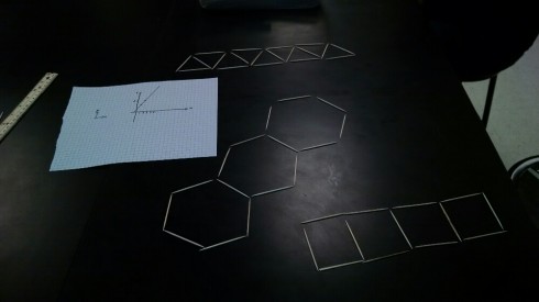
Toothpick shape sequences.

Using a sequence of connected shapes to introduce algebra and graphing to pre-Algebra students.

Make a geometric shape–a square perhaps–out of toothpicks. Count the sides–4 for a square. Now add another square, attached to the first. You should now have 7 toothpicks. Keep adding shapes in a line and counting toothpicks. Now you can:

  • make a table of shapes versus toothpicks,
  • write the sequence as an algebraic expression
  • graph the number of shapes versus the number of toothpicks (it should be a straight line),
  • figure out that the increment of the sequence–3 for a square–is the slope of the line.
  • show that the intercept of the line is when there are zero shapes.

Then I had my students set up a spreadsheet where they could enter the number of shapes and it would give the number of toothpicks needed. Writing a small program to do the same works is the next step.

Embedding more Graphs (using Flot)

Here’s another attempt to create embeddable graphs of mathematical functions. This one allows users to enter the equation in text form, has the option to enter the domain of the function, and expects there to be multiple functions plotted at the same time. Instead of writing the plotting functions myself I used the FLOT plotting library.

Profits per Explosion: An application of Linear Regression

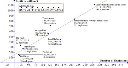
[Michael Bay] earns approximately 3.2 million $ for every explosion in his movies and a Michael Bay movie without explosions would earn 154.4 million $. This means that if Michael Bay wants to make a movie that earns more than Avatar’s 2781.5 million $ he has to have 817 explosions in his movie.

— Reddit:User:Mike-Dane: Math and Movies on Imgur.com.

There seems to be a linear relationship between the number of explosions in Michael Bay movies and their profitability. Graph by Reddit:User:Mike-Dane.

Reddit user Mike-Dane put together these entertaining linear regressions of a couple directors’ movie statistics. They’re a great way of showing algebra, pre-algebra, and pre-calculus students how to interpret graphs, and a somewhat whimsical way of showing how math can be applied to the fields of art and business.

Linear regression matches the best fit straight-line equations to data. The general equation for a straight line is:

y = mx + b

where m is the slope of the line — how fast in increases or decreases == and b is the intercept on the y-axis — which gives the initial value of the function.

So, for example, the Micheal Bay, profits vs. explosions, linear equation is:

Profit (in $millions) = 3.2 × (# of explosions) + 154

which means that a Michael Bay movie with no explosions (where # of explosions= 0) would make $154 million. And every additional explosion in a movie adds $3.2 million to the profits.

Furthermore, the regression coefficient (R2) of 0.89 shows that this equation is a pretty good match to the data.

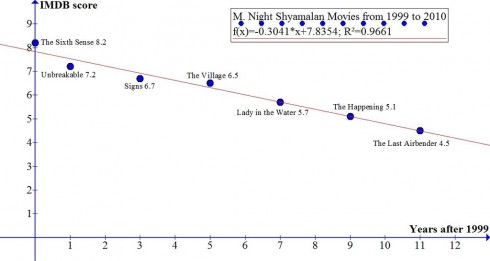
Mike-Dane gets an even better regression coefficient (R2 = 0.97) when he compares the quality of M. Night Shyamalan over time.

The scores of different M. Night Shyamalan movies calculated from user input on the Internet Movie DataBase (IMDB) decreases over time. Graph by Reddit:User:Mike-Dane.

In this graph the linear regression equation is:

Movie Score = -0.3014 × (year after 1999) + 7.8354

This equations suggests that the quality of Shyamalan’s movies decreases (notice the negative sign in the equation) by 0.3014 points every year. If you wanted to, you could, using some basic algebra, determine when he’d score a 0.

Embeddable Graphs

Going beyond just polynomials, I’ve created a javascript graphing app that’s easily embeddable.

At the moment, it just does polynomials and points, but polynomials can be used to teach quadratic functions (parabolas) and straight lines to pre-algebra and algebra students. Which I’ve been doing.

Based on my students’ feedback, I’ve made it so that when you change the equation of the line the movement animates. This makes it much easier to see what happens when, for example, you change the slope of a line.

P.S. You can also turn off the interactivity if you just want to show a simple graph. y = x2-1 is shown below:

Introducing Polynomials

If you recall, straight lines have a general equation that looks like this:

y=mx+b (1)

This is called the slope-intercept form of the equation, because m gives the slope, and b tells where the line intercepts the y-axis. For example the line:

y=2x-3 (2)

looks like:

Now, in the slope-intercept form, m and b represent numbers. In our example, m = 2 and b = 3.

So what if, instead of calling them m and b we used the same letter (let’s use a) and just gave two different subscripts so:

m = a_1 and,
b = a_0

therefore equation (1):

y=mx+b

becomes:
y = a_1 x + a_0 (3)

Now, in case you’re wondering why we picked m = a1 instead of m = a0, it’s because of the exponents of x. You see, in the equation x has an exponent of 1, and the constant b could be thought to be multiplying x with an exponent of 0. Considering this, we could rewrite our equation of the line (2):

y=2x^1-3x^0 (4)

since:
x^1 = x and,
x^0 = 1

we get:
y=2x-3(1)
y=2x-3

So in equation (3) the subscript refers to the exponent of x.

Now we can expand this a bit more. What if we had a term with x2 in an equation:

y=\frac{1}{2}x^2 + 2x - 3 (5)

Now we have three coefficients:

a_0 = -3 ,
a_1 = 2 and,
a_2 = \frac{1}{2} ,

And the graph would look like this.

Because of the x2 term (specifically because it has the highest exponent in the equation), this is called a second-order polynomial — that’s why the graph above has a little input box where the order is 2. In fact, on the graph above, you can change the order to see how the equation changes. Indeed, you can also change the coefficients to see how the graph changes.

A second order polynomial is a parabola, while, as you’ve probably guessed, a first order polynomial is a straight line. What’s a zero’th order polynomial?

Finally, we can write a general equation for a polynomial — just like we have the slope-intercept form of a line — using the a coefficients like:

y = a_n x^n + ... + a_2 x^2 + a_1 x + a_0

You can use the graphs to tinker around and see what different order polynomials look like, and how changing the coefficients change the graphs. I sort-of like the one below:

References

WolframAlpha has more details on polynomials.

The embedded graphs come from my own Polynomial Grapher.