Demonstrating Taylor Series Approximations with Graphs

This little embeddable, interactive app uses nth order polynomials to approximate a few curves to demonstrate the Taylor Series.

Numerical and Analytical Solutions 2: Constant Acceleration

Previously, I showed how to solve a simple problem of motion at a constant velocity analytically and numerically. Because of the nature of the problem both solutions gave the same result. Now we’ll try a constant acceleration problem which should highlight some of the key differences between the two approaches, particularly the tradeoffs you must make when using numerical approaches.

The Problem

A ball starts at the origin and moves horizontally with an acceleration of 0.2 m/s². Print out a table of the ball’s position (in x) with time (every second) for the first 20 seconds.

Analytical Solution
We know that acceleration (a) is the change in velocity with time (t):

$a = \frac{dv}{dt}$

so if we integrate acceleration we can find the velocity. Then, as we saw before, velocity (v) is the change in position with time:

$v = \frac{dx}{dt}$

which can be integrated to find the position (x) as a function of time.

So, to summarize, to find position as a function of time given only an acceleration, we need to integrate twice: first to get velocity then to get x.

For this problem where the acceleration is a constant 0.2 m/s² we start with acceleration:

$\frac{dv}{dt} = 0.2$

which integrates to give the general solution,

$v = 0.2 t + c$

To find the constant of integration we refer to the original question which does not say anything about velocity, so we assume that the initial velocity was 0: i.e.:

at t = 0 we have v = 0;

which we can substitute into the velocity equation to find that, for this problem, c is zero:

$v = 0.2 t + c$
$0 = 0.2 (0) + c$
$0 = c$

making the specific velocity equation:
$v = 0.2 t$

we replace v with dx/dt and integrate:

$\frac{dx}{dt} = 0.2 t$
$x = \frac{0.2 t^2}{2} + c$
$x = 0.1 t^2 + c$

This constant of integration can be found since we know that the ball starts at the origin so

at t = 0 we have x = 0, so;

$x = 0.1 t^2 + c$
$0 = 0.1 (0)^2 + c$
$0 = c$

Therefore our final equation for x is:

$x = 0.1 t^2$

Summarizing the Analytical

To summarize the analytical solution:

$a = 0.2$
$v = 0.2 t$
$x = 0.1 t^2$

These are all a function of time so it might be more proper to write them as:

$a(t) = 0.2$
$v(t) = 0.2 t$
$x(t) = 0.1 t^2$

Velocity and acceleration represent rates of change which so we could also write these equations as:

$a(t) = \frac{dv}{dt} = 0.2$
$v(t) = \frac{dx}{dt} = 0.2 t$
$x(t) = x = 0.1 t^2$

or we could even write acceleration as the second differential of the position:

$a(t) = \frac{d^2x}{dt^2} = 0.2$
$v(t) = \frac{dx}{dt} = 0.2 t$
$x(t) = x = 0.1 t^2$

or, if we preferred, we could even write it in prime notation for the differentials:

$a(t) = x''(t) = 0.2$
$v(t) = x'(t) = 0.2 t$
$x(t) = x(t) =0.1 t^2$

The Numerical Solution

As we saw before we can determine the position of a moving object if we know its old position (x_old) and how much that position has changed (dx).

$x_{new} = x_{old} + dx$

where the change in position is determined from the fact that velocity (v) is the change in position with time (dx/dt):

$v = \frac{dx}{dt}$

which rearranges to:

$dx = v dt$

So to find the new position of an object across a timestep we need two equations:

$dx = v dt$
$x_{new} = x_{old} + dx$

In this problem we don’t yet have the velocity because it changes with time, but we could use the exact same logic to find velocity since acceleration (a) is the change in velocity with time (dv/dt):

$a = \frac{dv}{dt}$

which rearranges to:

$dv = a dt$

and knowing the change in velocity (dv) we can find the velocity using:

$v_{new} = v_{old} + dv$

Therefore, we have four equations to find the position of an accelerating object (note that in the third equation I’ve replaced v with v_new which is calculated in the second equation):

$dv = a dt$
$v_{new} = v_{old} + dv$
$dx = v_{new} dt$
$x_{new} = x_{old} + dx$

These we can plug into a python program just so:

motion-01-both.py

from visual import *

# Initialize
x = 0.0
v = 0.0
a = 0.2
dt = 1.0

# Time loop
for t in arange(dt, 20+dt, dt):

     # Analytical solution
     x_a = 0.1 * t**2

     # Numerical solution
     dv = a * dt
     v = v + dv
     dx = v * dt
     x = x + dx

     # Output
     print t, x_a, x

which give output of:

>>> 
1.0 0.1 0.2
2.0 0.4 0.6
3.0 0.9 1.2
4.0 1.6 2.0
5.0 2.5 3.0
6.0 3.6 4.2
7.0 4.9 5.6
8.0 6.4 7.2
9.0 8.1 9.0
10.0 10.0 11.0
11.0 12.1 13.2
12.0 14.4 15.6
13.0 16.9 18.2
14.0 19.6 21.0
15.0 22.5 24.0
16.0 25.6 27.2
17.0 28.9 30.6
18.0 32.4 34.2
19.0 36.1 38.0
20.0 40.0 42.0

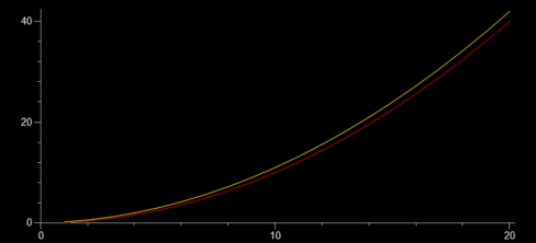
Here, unlike the case with constant velocity, the two methods give slightly different results. The analytical solution is the correct one, so we’ll use it for reference. The numerical solution is off because it does not fully account for the continuous nature of the acceleration: we update the velocity ever timestep (every 1 second), so the velocity changes in chunks.

To get a better result we can reduce the timestep. Using dt = 0.1 gives final results of:

18.8 35.344 35.532
18.9 35.721 35.91
19.0 36.1 36.29
19.1 36.481 36.672
19.2 36.864 37.056
19.3 37.249 37.442
19.4 37.636 37.83
19.5 38.025 38.22
19.6 38.416 38.612
19.7 38.809 39.006
19.8 39.204 39.402
19.9 39.601 39.8
20.0 40.0 40.2

which is much closer, but requires a bit more runtime on the computer. And this is the key tradeoff with numerical solutions: greater accuracy requires smaller timesteps which results in longer runtimes on the computer.

Post Script

To generate a graph of the data use the code:

from visual import *
from visual.graph import *

# Initialize
x = 0.0
v = 0.0
a = 0.2
dt = 1.0

analyticCurve = gcurve(color=color.red)
numericCurve = gcurve(color=color.yellow)
# Time loop
for t in arange(dt, 20+dt, dt):

     # Analytical solution
     x_a = 0.1 * t**2

     # Numerical solution
     dv = a * dt
     v = v + dv
     dx = v * dt
     x = x + dx

     # Output
     print t, x_a, x
     analyticCurve.plot(pos=(t, x_a))
     numericCurve.plot(pos=(t,x))

which gives:

Comparison of numerical and analytical solutions using a timestep (dt) of 1.0 seconds.

Numerical versus Analytical Solutions

We’ve started working on the physics of motion in my programming class, and really it boils down to solving differential equations using numerical methods. Since the class has a calculus co-requisite I thought a good way to approach teaching this would be to first have the solve the basic equations for motion (velocity and acceleration) analytically–using calculus–before we took the numerical approach.

Constant velocity

Question 1. A ball starts at the origin and moves horizontally at a speed of 0.5 m/s. Print out a table of the ball’s position (in x) with time (t) (every second) for the first 20 seconds.

Analytical Solution:
Well, we know that speed is the change in position (in the x direction in this case) with time, so a constant velocity of 0.5 m/s can be written as the differential equation:

$\frac{dx}{dt} = 0.5$

To get the ball’s position at a given time we need to integrate this differential equation. It turns out that my calculus students had not gotten to integration yet. So I gave them the 5 minute version, which they were able to pick up pretty quickly since integration’s just the reverse of differentiation, and we were able to move on.

Integrating gives:

$x = 0.5t + c$

which includes a constant of integration (c). This is the general solution to the differential equation. It’s called the general solution because we still can’t use it since we don’t know what c is. We need to find the specific solution for this particular problem.

In order to find c we need to know the actual position of the ball is at one point in time. Fortunately, the problem states that the ball starts at the origin where x=0 so we know that:

at t = 0, x = 0

So we plug these values into the general solution to get:

$0 = 0.5(0) + c$
solving for c gives:

$c = 0$

Therefore our specific solution is simply:

$x = 0.5t$

And we can write a simple python program to print out the position of the ball every second for 20 seconds:

motion-01-analytic.py

for t in range(21):
     x = 0.5 * t
     print t, x

which gives the result:

Numerical Solution:
Finding the numerical solution to the differential equation involves not integrating, which is particularly good if the differential equation can’t be integrated.

We start with the same differential equation for velocity:
$\frac{dx}{dt} = 0.5$

but instead of trying to solve it we’ll just approximate a solution by recognizing that we use dx/dy to represent when the change in x and t are really, really small. If we were to assume they weren’t infinitesimally small we would rewrite the equations using deltas instead of d’s:
$\frac{\Delta x}{\Delta t} = 0.5$

now we can manipulate this equation using algebra to show that:
$\Delta x = 0.5 \Delta t$

so the change in the position at any given moment is just the velocity (0.5 m/s) times the timestep. Therefore, to keep track of the position of the ball we need to just add the change in position to the old position of the ball:

$x_{new} = x_{old} + \Delta x$

Now we can write a program to calculate the position of the ball using this numerical approximation.

motion-01-numeric.py

from visual import *

# Initialize
x = 0.0
dt = 1.0

# Time loop
for t in arange(dt, 21, dt):
     v = 0.5
     dx = v * dt
     x = x + dx
     print t, x

I’m sure you’ve noticed a couple inefficiencies in this program. Primarily, that the velocity v, which is a constant, is set inside the loop, which just means it’s reset to the same value every time the loop loops. However, I’m putting it in there because when we get working on acceleration the velocity will change with time.

I also import the visual library (vpython.org) because it imports the numpy library and we’ll be creating and moving 3d balls in a little bit as well.

Finally, the two statements for calculating dx and x could easily be combined into one. I’m only keeping them separate to be consistent with the math described above.

A Program with both Analytical and Numerical Solutions
For constant velocity problems the numerical approach gives the same results as the analytical solution, but that’s most definitely not going to be the case in the future, so to compare the two results more easily we can combine the two programs into one:

motion-01.py

from visual import *
# Initialize
x = 0.0
dt = 1.0

# Time loop
for t in arange(dt, 21, dt):
     v = 0.5

     # Analytical solution
     x_a = v * t

     # Numerical solution
     dx = v * dt
     x = x + dx

     # Output
     print t, x_a, x

which outputs:

>>> 
1.0 0.5 0.5
2.0 1.0 1.0
3.0 1.5 1.5
4.0 2.0 2.0
5.0 2.5 2.5
6.0 3.0 3.0
7.0 3.5 3.5
8.0 4.0 4.0
9.0 4.5 4.5
10.0 5.0 5.0
11.0 5.5 5.5
12.0 6.0 6.0
13.0 6.5 6.5
14.0 7.0 7.0
15.0 7.5 7.5
16.0 8.0 8.0
17.0 8.5 8.5
18.0 9.0 9.0
19.0 9.5 9.5
20.0 10.0 10.0

Solving a problem involving acceleration comes next.

Volumes of Revolution

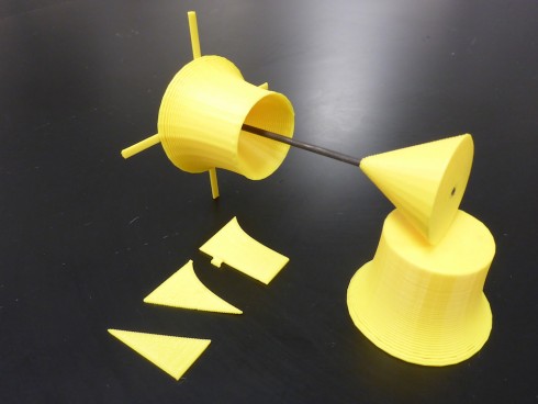
It can be tricky explaining what you mean when you say to take a function and rotate it about the x-axis to create a volume. So, I made an OpenScad program to make 3d prints of functions, including having it subtract one function from another. I also 3d printed a set of axes to mount the volumes on (and a set of cross-sections of the volumes being rotated.

The picture above are the functions Mrs. C. gave her calculus class on a recent worksheet. Specifically:

$y = e^{-x}+2$

from which is subtracted:

$y = 0.5 x$

A Visual Introduction to Differentiation (using vpython)

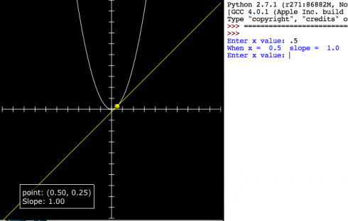
Screen capture: Enter an x value and the program calculates the slope for the function and draws the tangent line.

This quick program is intended to introduce differentiation as a way of finding the slope of a line. Students know how to find the slope of a tangent line at least conceptually (by drawing). We pick a curve: in this case:

$f(x) = x^2$

then enter values of x in the program to see how x, the function value and the differential compare to each other.

x	f(x)	f'(x)
0.5	0.25	1
1	1	2
2	2	4
3	9	6

Because it’s quick you have to change the function in the code, and enter the values for x in the python shell.

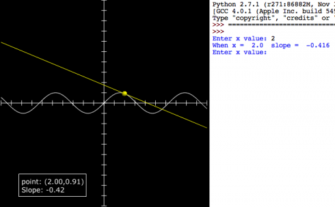
differentiation_intro_numeric.py

from visual import *

class tangent_line:
    def __init__(self):
        self.dx = 0.1
        self.line = curve()
        self.tangent_line = curve()
        self.point = sphere(radius=.25,color=color.yellow)
        self.point.visible = False
        self.label = label(pos=(-5,-8))

    '''CHANGE FUNCTION (y) HERE'''
    # the original function
    def f(self, x):
        #y = sin(x)
        y = x**2
        return y
    '''END CHANGE FUNCTION HERE'''

    def find_slope(self, x):
        sdx = .00001
        m = (self.f(x+sdx)-self.f(x))/sdx
        return round(m,3)
        
    def draw(self):
        for x in arange(xmin, xmax+self.dx, self.dx):
            self.line.append(pos=(x, self.f(x)))

    def draw_tangent(self, x):
        m = self.find_slope(x)
        y = self.f(x)
        b = y - m * x
        print "When x = ", x, " slope = ", m
        self.label.text = "point: (%1.2f, %1.2f)\nSlope: %1.2f" % (x,y,m)
        self.plot_point(x)

        #draw tangent
        self.tangent_line.visible = False
        self.tangent_line = curve(pos=[(xmin,m*xmin+b),(xmax,m*xmax+b)], color=color.yellow)
              
    def plot_point(self, x):
        self.point.visible = True
        self.point.pos = (x, self.f(x)) 

#axes
xmin = -10.
xmax = 10.
ymin = -10.
ymax = 10.
xaxis = curve(pos=[(xmin,0),(xmax,0)])
yaxis = curve(pos=[(0,ymin),(0,ymax)])

#tick marks
tic_dx = 1.0
tic_h = .5
for i in arange(xmin,xmax+tic_dx,tic_dx):
    tic = curve(pos=[(i,-0.5*tic_h),(i,0.5*tic_h)])
for i in arange(ymin,ymax+tic_dx,tic_dx):
    tic = curve(pos=[(-0.5*tic_h,i),(0.5*tic_h,i)])

#stop scene from zooming out too far when the curve is drawn
scene.autoscale = False

# draw curve
func = tangent_line()
func.draw()

# get input
while 1:
    xin = raw_input("Enter x value: ")
    func.draw_tangent(float(xin))

Differentiation Using Limits

We can use the idea of limits to come up with some general relationships between functions and their slopes. Take, for example, the last project where we found the slope of the function y = x² at the point where x = 3:

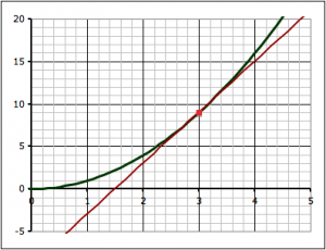
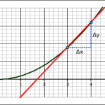
The green line is the curve y = x2 and the straight red line is the tangent to the curve at the point where x = 3 (i.e. at (3,9)). — The green line is the curve *y = x²* and the straight red line is the tangent to the curve at the point where *x = 3* (i.e. at (3,9)).

Finding the approximate slope using a forward difference.

We found the slope of the tangent line at the point (3,9) by a series of approximations. First we took two points on the curve, (3,9) and (4,16) and found the slope between those two points.

The equation for slope can be written in any of these three ways:

we find the exact slope by taking points on the line closer and closer together (which means that Δx is getting smaller and smaller). In math-speak, we’re saying that we’re taking the limit of the slope equation as Δx approaches zero.

Since we’re taking Δx to zero we might as well ask what happens to the slope when Δx is equal to zero.

As we can see from the equation, we end up with zero on the denominator, which makes the whole thing undefined, which we really do not want.

But what if we can rearrange things to get the Δx out of the denominator?

Let’s rewrite the equation y = x² as a function:

$f(x) = x^2$

So the point we’re interested in find the slope at is just (x, f(x)), which in this case happens to be (3, 9), but we’re not going to be using the actual numbers anymore so we can come up with a more general relationship.

To find the slope we find the point where the value on the x-axis is x and the value on the y-axis is f(x). — To find the slope we find the point where the value on the x-axis is x and the value on the y-axis is *f(x)*.

Now, and this is often the tricky part, the second point we use is going to have an x value of x + Δx:

For the second point, the x value we use is the first x offset by Δx.

which means that the value on the curve is f(x+Δx):

Our second point is where the x value is x+Δx and the y value is f(x+Δx). — Our second point is where the x value is *x+Δx* and the y value is *f(x+Δx)*.

So lets carefully observe the notation here. To find the slope of a line we can use the equation:

But with the function notation:

y₁ = f(x)
y₂ = f(x+Δx)

so:

Now watch very carefully as I replace the function notation with the actual functions, specifically:

f(x) = x²
f(x+Δx) = (x+Δx)²

to give:

and if you understand how this, we’re almost all there, because the rest is algebra.

We simplify the equation above by expanding the numerator.

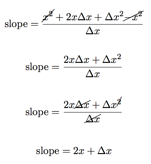
now we can subtract the similar terms (x²) and divide through by Δx to get:

But remember we don’t just want the slope, we want to find the slope where Δx approaches zero:

The problem before was that if we made Δx = 0 the equation would be undefined. But now, however, as Δx = 0 the second term in the equation just goes to zero:

leaving us just with the first term 2x:

Remember that we were trying to do this at the point where x = 3. So if we put x = 3 into this equation we get:

Which we know is the right answer because we did the very problem by hand already.

but now however we’ve come up with a more general equation for the slope. With it we can easily find the slope of our curve at any point along the curve!

For example, what is the slope of the curve when x = 0:

Notation

Now it’s a bit cumbersome to write the limit as Δx goes to zero every time, so we’ll instead call our equation for the slope of the line the differential, and we’ll give it the notation as the function prime:

i.e. if we have a function f(x) = x²:

we write its differential as:

To confuse things (at least for the moment) there are a number of ways of writing the differential (the different methods are useful in different contexts), so you will see things like:

So now that we know how to find the differential using limits, we’ll practice finding the differential of polynomial functions and see if we can find a general pattern that allows us to bypass the whole limits thing altogether.

Finding the Limit (Following up the Guitar Project)

Following up on the project to find the volume (and surface area) of a guitar, and the slope at a point along the outline of the guitar, I asked students to use the same techniques to estimate the area under a curve (y = x²) and find the slope at a point along the curve. Specifically:

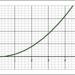
Draw the function y = x²
Find the area bounded by the function, the lines x = 1 and x = 4, and the x-axis
Find the slope of a tangent to the y = x² function at the point where x = 3.

The point of the second question is to test if students have internalized the idea that they can approximate curved shapes with trapezoids, but they have to weigh the time it will take to do a lot of trapezoids, versus the reduction in error that will result from more trapezoids. It’s interesting to see students’ character come through in this assignment: some choose to make one big trapezoid and are done, while other will go so many trapezoids that they run out of time to get them done.

It just occurs to me, however, that an interesting way to assess this assignment would be to give them a fixed time, and tell them that their score will be the 100 minus the percent error in their calculations.

Limits

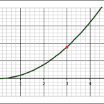
The third question–about finding the slope of a tangent line at x = 3–is our jumping off point into the mathematics of limits and calculus.

Some students do a single approximation–either forward or backward–, while others do both and take the average.

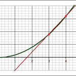
The forward approximation involves finding the values for the function y = x² at x = 3 and x = 4 and finding the slope between the two points:

when x = 3, y = 9, so we have the point (x₁,y₁) = (3, 9)
when x = 4, y = 16, so we have the point (x₂,y₂) = (3, 16)

The slope (m) between two points is found with the equation they learned back in algebra:

$\text{slope} = m = \frac{\Delta y}{\Delta x} = \frac{y_2-y_1}{x_2-x_1} = \frac{y_2-y_1}{\Delta x}$

Where Δx = x₂-x₁ and Δy = y₂-y₁.

Using the two points above gives:

$\text{slope} = m = \frac{\Delta y}{\Delta x} = \frac{16-9}{4-3} = \frac{7}{1} = 7$

Those who use the backward approximation simply use the point when x = 2 instead of x = 4, and they end up with a value for the slope of 5.

Averaging the forward and backward approximations give a slope of 6.

Now, since they know that the closer you make the points the better the approximation, I ask them to make a table to see what happens as they do so. This means reducing the value of Δx. In both the forward and backward approximation shown above, Δx = 1.

This can be done very quickly in Excel (or any other spreadsheet program), however, this time at least, most students chose to do it by hand. They end up with a table that looks like this:

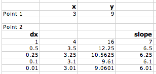
As dx gets smaller the calculated slope approaches 6.

As the difference in x gets smaller and approaches zero, the slope approaches 6.

As you plot slope versus the change in x (Δx), you can see that as Δx gets smaller and smaller and approaches zero, the slope gets closer and closer to 6. So we could say that:

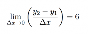
the limit of the slope as Δx approaches zero is 6.

Mathematically this can be written as:

or using the equation for slope:

Now, we can work on taking the limit in a more general way to do differentiation.

Introducing Limits (Calculus) with a Guitar

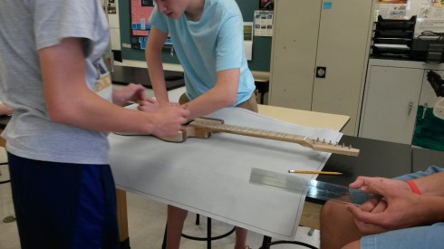
One of the assigned tasks from last summer’s guitar building workshop was to create a few modules for use in class. I worked on an assignment that has students calculate the volume of a guitar body using trapezoidal approximation methods that can be a bridge between pre-calculus and calculus.

The first draft of this module is here: volume-activity-v01.pdf (the LaTeX file is volume-activity-v01.tex.zip ). It has made contact with the ~~enemy~~ students and the results have so far been very good.

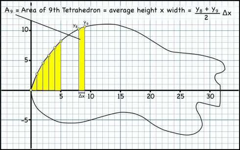
A method for finding the area of a guitar body by fitting trapezoids.

There were two things that I need to add for next time:

How to find the area of a trapezoid: I should have some more detail about how I came up with the formula for calculating the area of each trapezoid (see the figure above). I multiply the average of the heights of the two sides of the trapezoid by the width of the base to get the area. Students tend to want to find the area of the lower rectangle, then add the area of the upper triangle. Their method gives the same answer for area, but results in a more complicated equation that takes more effort to generalize.
Have them also find the slope of a tangent line to the outline of the guitar at a certain point. This assignment is intended to lead students up to the concept of limits with the idea that if you make the trapezoids thinner you’ll get less error in your calculation of the total area. So, as the width of the trapezoid approaches zero, you should get the exact area (with no error). The seemed to get that fairly well, however, when I get into the calculus, I actually first use limits to show them how to find derivatives of functions before I talk about finding areas under curves. As a result, I did ask the students to find the slope at a point on their guitar outline (I randomly chose a point from their outlines), and was very glad I did so. This should be included in the module.

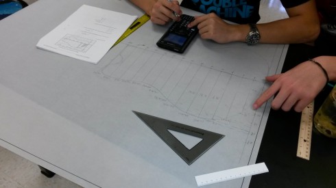
Students drawing trapezoids to fit the outline of the guitar, and calculating their areas.

Finally, in addition, I also showed them how to quickly calculate the trapezoid areas once they’d entered the coordinates of each point on their graphs into Excel. I did not test them on this afterward, so I’m not sure how much of it they absorbed.