In which we follow the path of a raindrop from the watershed’s divide to its estuary on the lake.

The most recent immersion. Coon Creek.
We stayed at Natchez Trace State Park and just a couple meters away from the villas is the head of the Oak Ridge Trail (detailed park map here).
View Natchez Trace Immersion Hike in a larger map
The first thing you notice is a small, rickety bridge whose main job is to keep your feet dry as you cross a very small stream. The stream is on its delta, so the ground is very soggy, and the channel is just about start its many bifurcations into distributaries that fan out and create the characteristic deltaic shape.

There’s a bright orange flocculate on the quieter parts of the stream bed. It’s the color of fresh rust, which leads me to suspect it’s some sort of iron precipitate.

Iron minerals in the sediments and bedrock of the watershed are dissolved by groundwater, but when that water discharges into the stream it becomes oxygenated as air mixes in. The dissolved iron reacts with the oxygen to create the fine orange precipitate. Sometimes, the chemical reaction is abiotic, other times it’s aided by bacteria (Kadlec and Wallace, 2009).

Past the small delta, the trail follows the lake as it curves around into another, much bigger estuary (see map above). We found much evidence of flora and fauna, including signs of beavers.
We even took the time to toss some sticks into the water to watch the waves. With a single stick, you can see the wave dissipate as it expands, much like I tried to model for the height of a tsunami. We also threw in multiple sticks to create interference patterns.

The Oak Ridge Trail, which we followed, diverges from the somewhat longer Pin Oak Trail at the large estuary (which is marked on the map). The Pin Oak Trail takes you through some beautiful stands of conifers, offering the chance to talk about different ecological communities, but we did not have the time to see both trails.
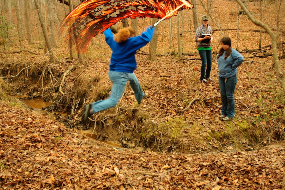
Instead, we followed the Oak Ridge Trail up the ridge (through one small stand of pines) until it met the road. The road is on the other side of the watershed divide. I emphasized the concept by having my students stand in a line across the divide and point in the direction of that a drop of water, rolling across the ground, would flow.

Then I told them that we’d get back by following our fictitious water droplet off the ridge into the valley. And we did, traipsing through the leaf-carpeted woods.

Of course there were no water droplets flowing across the surface. Unless its actively raining, water tends to sink down into the soil and flow through the ground until it gets to the bottom of the valley, where it emerges as springs. Even before you see the first spring, though, you can see the gullies carved by overland flow during storms.

Following the small stream was quite enjoyable. It was small enough to jump across, and there were some places where the stream had bored short sections of tunnels beneath its bed.

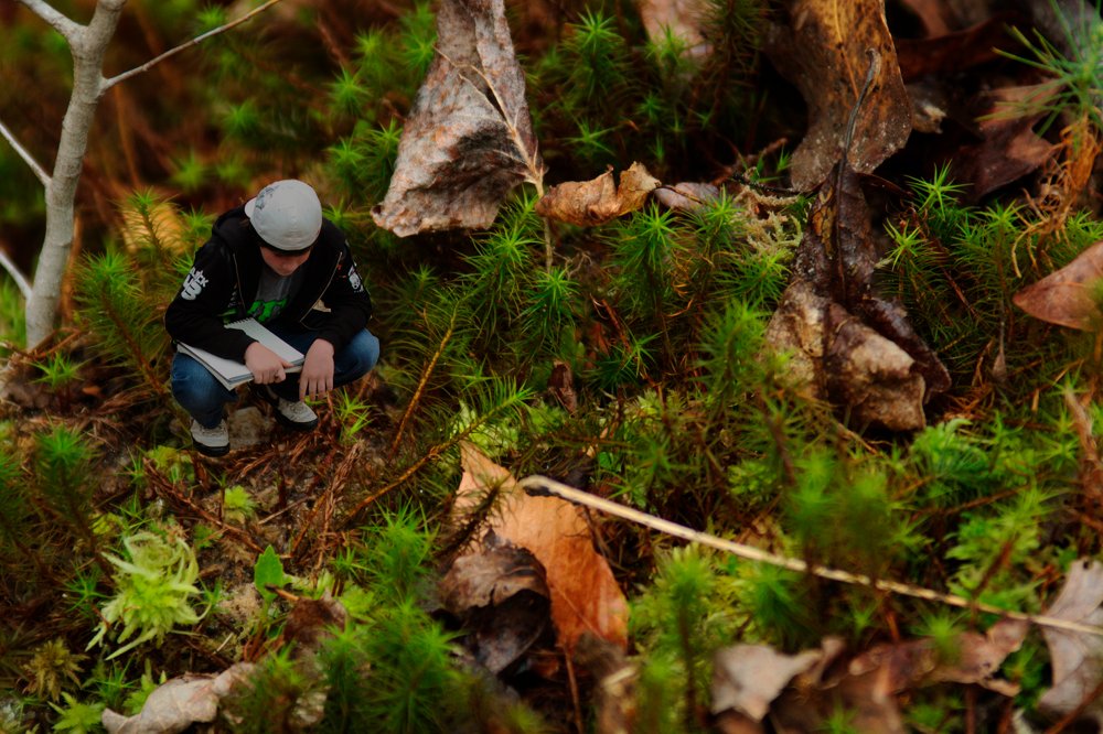
I took the time to observe the beautiful moss that maintained the banks of the stream. Students took the time to observe the environment.

Downstream the valley got wider and wider, and the stream cut deeper and deeper into the valley floor, but even the small stream sought to meander back and forth, creating beautiful little point bars and cut-banks.

As the stream approached its estuary it would stagnate in places. There, buried leaves and organic matter would decay under the sediment and water in anoxic conditions, rendering their oils and producing natural gas. We’re going to be talking about global warming and the carbon cycle next week so I was quite enthused when students pointed out the sheen of oils glistening on isolated pools of stagnant water.

Finally, we returned to the estuary. It’s much larger than the first one we saw, and it’s flat, swampy with lots of distributaries, and chock full of the sediment and debris of the watershed above it.

This less than three kilometer hike took the best part of two hours. But that’s pretty fast if you value your dawdling.


