The first 10 videos in this series explain where the idea of imaginary numbers come from, how the complex plane makes finding roots easier, and how imaginary numbers are needed for closure in algebra.
Tag: algebra
Calculating π
A very good explanation of how Newton applied calculus to come up with a much more efficient method of calculating pi (π). It starts with a nice illustration of the relationship between π and the area of a circle, moves explains the binomial theorem (quite nicely), and then shows how Newton generalized the binomial theorem to come up with an integral of a quarter of a unit circle. They don’t explain what a unit circle is, but that’s easy: it’s just a circle with a radius of 1.
Gaga Ball Pit

A couple middle-schoolers decided to build a gaga ball pit for their interim project. Since they’d already had their plan improved and I’d picked up the wood over the weekend, they figured they could get it done in a day or two and then move on to other things for the rest of the week. However, it turned out to be a bit more involved.
They spent most of their first day–they just had afternoons to work on this project–figuring out where to build the thing. It’s pretty large, and our head-of-school was in meetings all afternoon, so there was a lot of running back and forth.
The second day involved some math. Figuring out where to put the posts required a little geometry to determine the internal angles of an octagon, and some algebra (including Pythagoras’ Theorem) to calculate the distance across the pit. The sum a2 + a2 proved to be a problem, but now that they’ve had to do it in practice they won’t easily forget that it’s not a4.
Mounting the rails on the posts turned out the be the main challenge on day three. They initially opted for trying to drill the rails in at an angle, but found out pretty quickly that that was going to be extremely difficult. Eventually, they decided to rip the posts at a 45 degree angle to get the 135 degree outer angle they needed. We ran out of battery power for the saw and our lag screws were too long for the new design, so assembly would have to wait another day.
Finally, on day four they put the pit together. It only took about an hour–they’d had the great idea on day three to put screws into the posts at the right height, so that they could rest the rails on the screws to hold them into place temporarily as they mounted the rails. By the time they added the final side the octagon was only off by a few, easily adjusted centimeters.
They did an excellent job and noted, in our debrief, just how important the planning was, even though it was their least favorite part of the project. I’d call it a successful project.
A First Program
Working on algebra over the summer, we tried a little programming. This is O’s first program, which gives the chirp rate of crickets based on the temperature.
t = float(raw_input('enter temperature> '))

n=4*t-160
print "number of chirps=", n
print "t=", t
Embedding more Graphs (using Flot)
Here’s another attempt to create embeddable graphs of mathematical functions. This one allows users to enter the equation in text form, has the option to enter the domain of the function, and expects there to be multiple functions plotted at the same time. Instead of writing the plotting functions myself I used the FLOT plotting library.
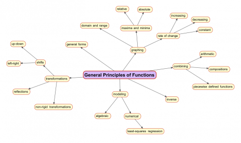
A Concept Map for Mathematical Functions
This year I’m trying teaching pre-Calculus (and it should work for some parts of algebra as well) based on this concept map to use as a general way of looking at functions. Each different type of function can by analyzed by adapting the map. So linear functions should look like this:
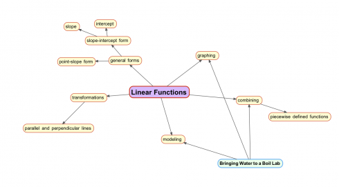
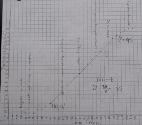
You’ll note the bringing water to a boil lab at the bottom left. It’s an adaptation of the melting snow lab my middle schoolers did. For the study of linear equations we’ll define the function using piecewise defined functions.
Profits per Explosion: An application of Linear Regression
[Michael Bay] earns approximately 3.2 million $ for every explosion in his movies and a Michael Bay movie without explosions would earn 154.4 million $. This means that if Michael Bay wants to make a movie that earns more than Avatar’s 2781.5 million $ he has to have 817 explosions in his movie.
— Reddit:User:Mike-Dane: Math and Movies on Imgur.com.
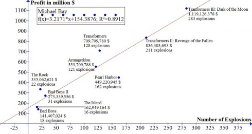
Reddit user Mike-Dane put together these entertaining linear regressions of a couple directors’ movie statistics. They’re a great way of showing algebra, pre-algebra, and pre-calculus students how to interpret graphs, and a somewhat whimsical way of showing how math can be applied to the fields of art and business.
Linear regression matches the best fit straight-line equations to data. The general equation for a straight line is:
y = mx + b
where m is the slope of the line — how fast in increases or decreases == and b is the intercept on the y-axis — which gives the initial value of the function.
So, for example, the Micheal Bay, profits vs. explosions, linear equation is:
Profit (in $millions) = 3.2 × (# of explosions) + 154
which means that a Michael Bay movie with no explosions (where # of explosions= 0) would make $154 million. And every additional explosion in a movie adds $3.2 million to the profits.
Furthermore, the regression coefficient (R2) of 0.89 shows that this equation is a pretty good match to the data.
Mike-Dane gets an even better regression coefficient (R2 = 0.97) when he compares the quality of M. Night Shyamalan over time.
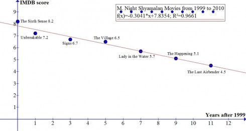
In this graph the linear regression equation is:
Movie Score = -0.3014 × (year after 1999) + 7.8354
This equations suggests that the quality of Shyamalan’s movies decreases (notice the negative sign in the equation) by 0.3014 points every year. If you wanted to, you could, using some basic algebra, determine when he’d score a 0.
Introducing Polynomials
If you recall, straight lines have a general equation that looks like this:
![]() (1)
(1)
This is called the slope-intercept form of the equation, because m gives the slope, and b tells where the line intercepts the y-axis. For example the line:
![]() (2)
(2)
looks like:
Now, in the slope-intercept form, m and b represent numbers. In our example, m = 2 and b = 3.
So what if, instead of calling them m and b we used the same letter (let’s use a) and just gave two different subscripts so:
![]() and,
and,
![]()
therefore equation (1):
![]()
becomes:
![]() (3)
(3)
Now, in case you’re wondering why we picked m = a1 instead of m = a0, it’s because of the exponents of x. You see, in the equation x has an exponent of 1, and the constant b could be thought to be multiplying x with an exponent of 0. Considering this, we could rewrite our equation of the line (2):
![]() (4)
(4)
since:
![]() and,
and,
![]()
we get:
![]()
![]()
So in equation (3) the subscript refers to the exponent of x.
Now we can expand this a bit more. What if we had a term with x2 in an equation:
![]() (5)
(5)
Now we have three coefficients:
![]() ,
,
![]() and,
and,
![]() ,
,
And the graph would look like this.
Because of the x2 term (specifically because it has the highest exponent in the equation), this is called a second-order polynomial — that’s why the graph above has a little input box where the order is 2. In fact, on the graph above, you can change the order to see how the equation changes. Indeed, you can also change the coefficients to see how the graph changes.
A second order polynomial is a parabola, while, as you’ve probably guessed, a first order polynomial is a straight line. What’s a zero’th order polynomial?
Finally, we can write a general equation for a polynomial — just like we have the slope-intercept form of a line — using the a coefficients like:
![]()
You can use the graphs to tinker around and see what different order polynomials look like, and how changing the coefficients change the graphs. I sort-of like the one below:
References
WolframAlpha has more details on polynomials.
The embedded graphs come from my own Polynomial Grapher.
