A Study in Linear Equations

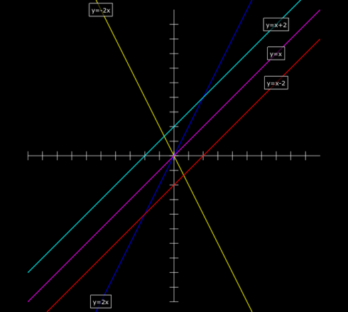
The effects of changing the constants in the equation of a line (y=mx+b). Image by Tess R.

My high school pre-Calculus class is studying the subject using a graphical approach. Since we’re half-way through the year I thought it would be useful to introduce some programming by building their own graphical calculators using Vpython.

Now, they all have graphical calculators, and Vpython does have its own graphing capabilities, but they’re fairly simple, only 2-dimensional, and way too automatic, so I prefer to have students program the calculators in full 3d space.

My approach to graphing is fairly simple too, but its nice because it introduces:

  • Co-ordinates: Primarily in 2d (co-ordinate plane), but 3d is easy;
  • Lists: in this case its a list of coordinates on a line;
  • Loops: (specifically for loops) to repeat actions and produce a sequence of numbers (with range); and
  • A sideways glance at matrix-like operations with arrays: A list of numbers can be treated like a matrix in some relatively simple circumstances. However, it’s not real matrix operations: multiplying a scalar by a list works like real matrix multiplication, but multiplying two lists multiplies the corresponding elements in the list.

A Simple Graphing Program

Start the program with the standard vpython header:

from visual import *

x and y axes: curves and lists

Next create the x and y axes. This introduces the curve object and lists, because Vpython draws its curve from a series of points held in a list.

To keep things simple, we’re letting the graph go from -10 to positive 10 along both axes, which makes the x-axis a line segment with only two points:

line_segment = [(-10,0), (10,0)]

The square brackets say that what’s inside as a list. In this case it’s a list of two coordinate pairs, (-10,0) and (10,0).

Now we create a line using Vpython’s curve and tell it that the positions of the points on the curve are the ones we just defined:

xaxis = curve(pos=line_segment)

To create the y-axis, we do the same thing but change the coordinate pair to (0,-10) and (0,10).

line_segment = [(0,-10),(0,10)]
yaxis = curve(pos=line_segment)

Which should produce:
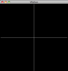
Very simple x and y axes.

Tic-marks: loops

In order to be better able to keep track of things, we’ll need some tic-marks on the axes. Ideally we’d like to label them too, but I think it works well enough to save that for later.

I start by having students create the first few tic-marks and then look for the emerging pattern. Their first attempts usually look something like this:

mark1 = curve(pos=[(-10,0.3),(-10,-0.3)])
mark2 = curve(pos=[(-9,0.3),(-9,-0.3)])
mark3 = curve(pos=[(-8,0.3),(-8,-0.3)])
mark4 = curve(pos=[(-7,0.3),(-7,-0.3)])
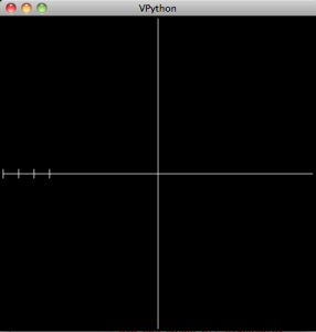
A few tic marks.

However, instead of tediously writing out these lines we can automate it by noticing that the only things that change are the x-coordinate of the coordinate pairs: they go from -10, to -9, to -8 etc.

So we want to produce a set of numbers that go from -10 to 10, in increments of 1, and use those number to make the tic-marks. The range function will do just that: specifically, range(-10,10,1). Actually, this list only goes up to 9, but that’s okay for now.

We tell the program to go through each item in the list and give its value to the variable i using a for loop:

for i in range(-10,10,1):
    mark = curve(pos=[(i,0.3),(i,-0.3)])

In python, everything indented after the for statement is within the loop.
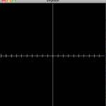
Tic marks on the x-axis.

The y-axis’ tic-marks are similar, and its a nice little challenge for students to figure them out. They usually come up with a separate loop, eventually, that looks something like:

for i in range(-10,10,1):
    mark = curve(pos=[(0.3, i),(-0.3,i)])
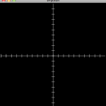
Our axes.

The Curve

Now to create a line we really only need two points. However, so that we can make other types of curves later on we’ll create a line with a series of points. We’ll create the x and y values separately:

First we set up the set of x values:

line = curve(x=arange(-10,10,0.1))

Note that I use the arange function which is just like the range function but gives you decimal values (so you can do fractions) instead of just integers.

Next we set the y values that go with the x values for the equation (in this example):
! y = 0.5 x + 2

line.y = 0.5 * line.x + 2

Finally, to make it look better, we change the color of the line to yellow:

line.color = color.yellow

In Summary

The final code looks like:

from visual import *


line_segment = [(-10,0),(10,0)]
xaxis = curve(pos=line_segment)

line_segment = [(0,-10),(0,10)]
yaxis = curve(pos=line_segment)

mark1 = curve(pos=[(-10,0.3),(-10,-0.3)])
mark2 = curve(pos=[(-9,0.3),(-9,-0.3)])
mark3 = curve(pos=[(-8,0.3),(-8,-0.3)])
mark4 = curve(pos=[(-7,0.3),(-7,-0.3)])

for i in range(-10,10,1):
    mark = curve(pos=[(i,0.3),(i,-0.3)])

for i in range(-10,10,1):
    mark = curve(pos=[(0.3, i),(-0.3,i)])


line = curve(x=arange(-10,10,0.1))
line.y = 0.5 * line.x + 2
line.color = color.yellow

which produces:
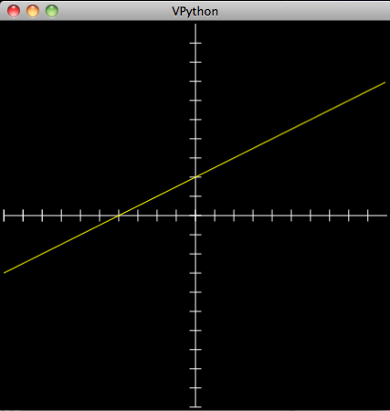
A first line: y=0.5x+2

Note on lists, arrays and matrices: You’ll notice that we create the curve, give it a list of x values (using arange), and then calculate the corresponding y values using matrix multiplication: 0.5 * line.x. This works because line.x actually stores the values as an an array, not as a list. The key difference between lists and arrays, as far as we’re concerned, is that we can get away with this type of multiplication with an array and not a list. However, an array is not a matrix, as is clearly demonstrated by the second part of the command where 2 is added to the result of the multiplication. In this case, 2 is added to each value in the array; if it were an actual matrix you need to add another matrix of the same shape that’s filled with 2’s. Right now, this is invisible to the students. The line of code makes sense. The concern is that when they do start working with matrices there might be some confusion. So watch out.

And to make any other function you just need to adjust the final line. So a parabola:
! y = x^2
would be:

line.y = line.x**2

(The two stars “**” indicates an exponent).

An Assignment

So, to assess learning, and to review the different functions we’ve learned, I asked students to produce “studies” of the different curves by demonstrating what happens when you change the different constants and coefficients in the equation.

For a straight line the general equation is:
! y = mx + b

you what happens when:

  • m > 1;
  • 0 < m < 1;
  • m < 0

and:

  • b > 1;
  • 0 < b < 1;
  • b < 0

The result is, after you add some labels, looks something like the image at the very top of this post.

This type of exercise can be done for polynomials, exponential, trigonometric, and almost any other type of functions.

FOIL: Multiplying Factors

FOILing.

Multiplying out two factors can be a little tricky. The FOIL mnemonic is a quick method when you have two terms in each factor, such as in:

(a + b)(a + b)

FOIL stands for:

  • Firsts,
  • Outer,
  • Inner,
  • Lasts.

It applies to the multiplication of the binomial cube.

Multiplying out factors using FOIL.

Another way of showing the process — step by step — would be like this:

Multiplying factors using FOIL.

After FOILing you combine the similar terms:

Combining like terms to get the final result.

Using the Binomial Cube in Algebra

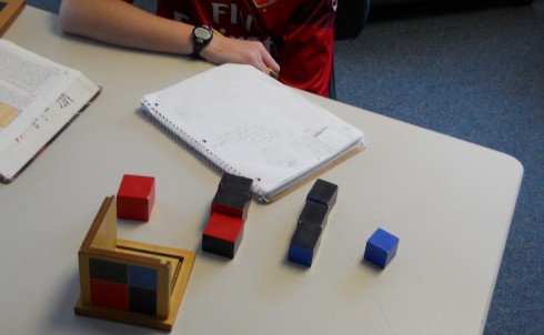
Figuring out (a+b)3; with a binomial cube.

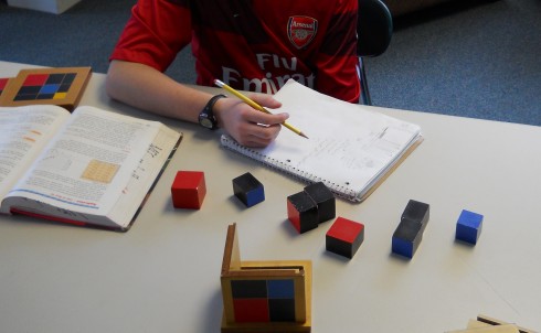
After working with the hundred-squares, ten-bars, and thousand-cubes to figure out how to add polynomials, we borrowed the binomial and trinomial cubes to practice multiplying out factors. It’s a physical way of showing factor multiplication.

Binomial Square

You can first look at the binomial cube in two-dimensions as a binomial square by just finding the area of the top layer of four blocks.

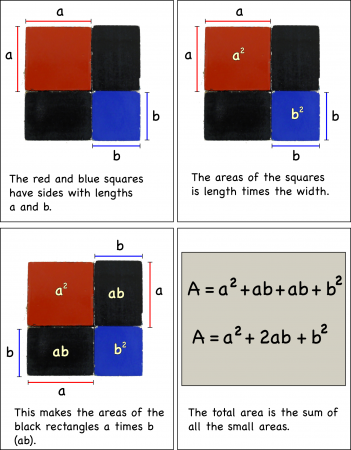
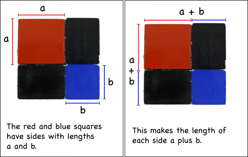
If you label the length of the side of the red block, a, and the length of the blue block, b, you can calculate the areas of the individual pieces simply by multiplying their lengths times their widths.

Looking from the top down, the top layer of the binomial cube is a binomial square.

Adding up the individual areas you get the area of the entire square:

A = a^2 + 2ab + b^2

However, there is another way.

If you recognize that the length of each side of the entire square is equal to (a+b).

The length of each side of the cube is the sum of the lengths of the two squares.

Then the total area is going to be total length (a+b) times the total width (a+b):

A = (a+b)^2 = (a+b)(a+b)

We can multiply this out (using FOIL is easiest):

(a+b)(a+b) = a^2 + ab + ab + b^2

which simplifies to give the same result as adding up the individual areas:

(a+b)^2 = a^2 + 2ab + b^2

The Binomial Cube

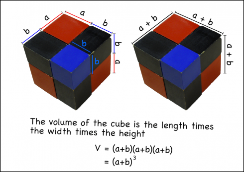
We can do the same thing using the entire cube by recognizing that the volume of the cube is the length times width times the depth, and all of these dimensions are the same: (a+b).

Using the full binomial cube.

Now the students can go through the same process of multiplying out the factors, and can check their work be seeing if they get the same number of pieces (and dimensions) as the physical cube.

Success!

Polynomials: Revisiting pre-Kindergarten

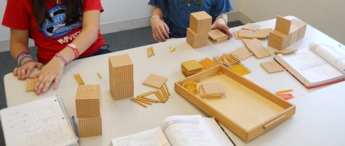
Working with the thousand cube, hundred square, ten bar and unit cells in algebra.

I sent a couple of my algebra students down to the pre-Kindergarten classroom to burrow one of their Montessori works. They were having a little trouble adding polynomials, and the use of manipulatives really helped.

The basic idea is that when you add something like:

 n^2 + 2n + 3n^2 + 4n + 5 + 2n^3 + 4 + 3n^3

you can’t add a n3 term to a n2 or a n term. You only combine the terms with the same degree (and same variables). So the equation above becomes:

 2n^3 + 3n^3 + n^2 + 3n^2 + 4n + 2n + 5 + 4

which simplifies to:

 5n^3 + 4n^2 + 6n + 9

The kids actually enjoyed the chance to run downstairs to burrow the materials from their old pre-K teacher (and weren’t they quite good about returning the materials when they were done with them).

And it clarifies a lot of misconceptions when you can clearly see that that you just can’t add a thousand cube to a ten bar — it just doesn’t work.

Parabolic Mirrors

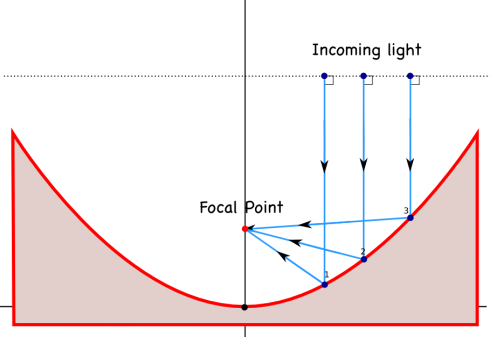
Parabolic mirrors magnify by reflecting parallel rays of incoming light onto a single point. (Adapted from Wikimedia Commons User:Nargopolis).

We’re talking about light and sound waves in physics at the moment, and NPR’s Morning Edition just had a great article on how the enormous, ultra-precise, mirrors that are used in large telescopes are made.

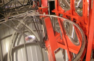
Astronomical observatories tend to use mirrors instead of lenses in their telescopes, largely because if you make lenses too big they tend to sag in the middle, while you can support a mirror all across the back, and because you have to make a lens perfect all the way through for it to work correctly, but only have to make one perfect surface for a parabolic mirror.

ScienceClarified has a great summary of the history of the Hubble Space telescope, that includes all the trouble NASA went through trying to fix it when they realized it was not quite perfect.

Large parabolic mirrors are used for magnification in telescopes. (Image via Wikipedia).

In addition, it’s interesting to note that you can also make a parabolic surface on a liquid by spinning it, resulting in liquid telescope mirrors .

Gravity, the Electromagnetic Forces, and the Inverse Square Law

Calculating the forces between two charged particles (electric force), two magnets (the magnetic force), and two masses (the gravitational force) require remarkably similar equations. But, while electricity and magnetism are directly related (that’s why it’s called electromagnetism), gravity is its own fundamental force. Yet they all depend (inversely) on the square of the distance between the two objects creating the force, so they’re all said to obey some form of the inverse square law.

Gravitational Force (Fg)

The force exerted by two masses on one another is:

 F_g = G \frac{m_1 m_2}{d^2}

where:

  • G is the gravitational constant (6.67300 × 10⁻¹¹ m3 kg-1 s-2
  • m1 and m2 are the masses of the two objects attracting one another.
  • d is the distance between the two objects.

Electrical Force (Fe)

The force exerted by two electrically charged objects on one another (like a proton and an electron), is:

 F_e = K \frac{q_1 q_2}{d^2}

where:

  • K is the electrical constant, sometimes called Coulumn’s constant (8.9876 × 10⁹ N m2 C-2
  • q1 and q2 are the sizes of the charges (in Coulumbs) of the two objects attracting one another.
  • d is the distance between the two objects.

Magnetic Force (Fm)

The force exerted by two magnets on one another, is:

 F_m = \mu \frac{p_1 p_2}{d^2}

where:

  • μ is a constant, (a little simplified)
  • p1 and p2 are strengths of the magnetic poles of the two objects attracting one another.
  • d is the distance between the two objects.

The magnetic force is a little more difficult to give a single equation for, because you need to factor in the shape of the magnets.

Inverse Square Laws

In addition to gravity, electric, and magnetic forces, light (which is electromagnetic radiation) and sound also obey inverse square laws.

Equations of a Parabola: Standard to Vertex Form and Back Again

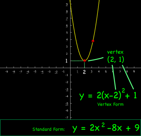
Highlighting the Vertex Form of the equation for a parabola.

The equation for a parabola is usually written as:

Standard form:
! y = ax^2 + bx + c

where a, b and c are constants. This is the form displayed in both the VPython Parabola and Excel parabola programs. However, to make the movement of the curve easier, the VPython program also uses the vertex form of the equation internally:

Vertex Form:
! y = a(x-h)^2 + k

where the point (h, k) is the location of the vertex of the parabola. In the example above, h = 1 and k = 2.

To translate between the two forms of the equation, you have to rewrite them. Start by expanding the vertex form:

y = a(x – h)2 + k

becomes:

y = a(x – h)(x – h) + k

multiplied out to get:

y = a(x2 – 2hx + h2) + k

now distribute the a:

y = ax2 – 2ahx + ah2 + k

finally, group all the coefficients:

y = (a)x2 – (2ah)x + (ah2 + k)

This equation has the same form as y = ax2 + bx + c if:

Vertex to Standard Form:

a = a
b = -2ah
c = ah2+k

And we can rearrange these equations to go the other way, to find the vertex form from the standard form:

Standard to Vertex Form:

! a = a
! h = \frac{\displaystyle -b}{\displaystyle 2a}
! k = c - ah^2 = c - \frac{\displaystyle b^2}{\displaystyle 4a}

Summary

In sum, you can write the standard equation for a parabola as:

Standard form:

And you can write the equation for the same parabola in vertex form as:

Vertex form:

UPDATES

UPDATE 1: This app will automatically convert from standard to vertex form (or back again).

UPDATE 2: Automatically generate and embed graphs using this parabolic grapher app.

Parabola Program

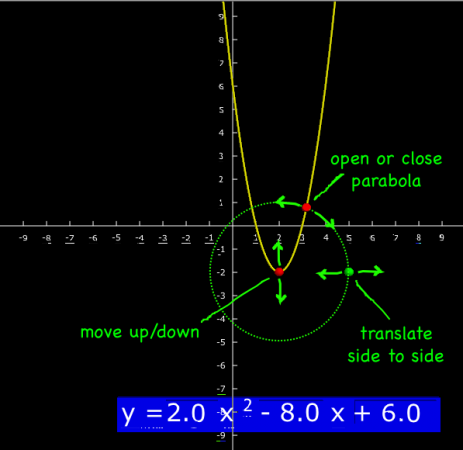
Animation showing the widening and shrinking of the parabola.

So I put together this interactive parabola program using VPython (code here) for students encountering these curves in Algebra.

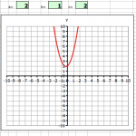
Simple Excel program to graph a parabola.

It’s a more interactive version of the Excel parabola program in that you can move the curve by dragging on some control points, rather than just having to enter the coefficients of the equation. The program is still in development, but it is at a useful stage right now, so I thought I’d make it available for anyone who wanted to try it.

The program is fairly straightforward to use. You can move the curve (translate it) up and down, and expand or tighten the area within the parabola.

The program also displays the equation of the curve in standard form:
! y = ax^2 + bx + c

.

What the buttons do.

Next Steps

I’m also working making the standard equation editable by clicking on it and typing, and am considering showing the x-axis intercepts, which will give algebra students a nice, visual way to of checking their factoring.

References

Coffman, J., 2011 (accessed). Translating Parabolas. http://www.jcoffman.com/Algebra2/ch5_3.htm

Math Warehouse, 2011 (accessed). Equation of a Parabola
Standard Form and Vertex Form Equations, http://www.mathwarehouse.com/geometry/parabola/standard-and-vertex-form.php#

WolframAlpha.com, 2011 (accessed). http://www.wolframalpha.com/input/?i=a^2+x^4%2Bx^2-r^2%3D0