Multi-modal IRP’s

If I present information to you orally, you’ll probably only remember about 10% 72 hours after exposure, but if I add a picture, recall soars to 65%.

–Alex Lundry (2009): Chart Wars: The Political Power of Data Visualization

How you present visual information is important. And my students are discovering this as they work up their Independent Research Projects (IRP’s) this week.

In the spring they are fairly free to pick their topic and style of IRP. Some choose research projects, others term papers, and a few do things that strike their fancy, like writing fiction or programming games.

In the end, they submit a written report and give a presentation.

For research projects, I have one student who did a great job of coming up with a hypothesis and testing it. He even compiled a nice table of his data for his results section, but was reluctant to go through the effort of making a graph. After all, he claimed, anyone reading his report (or watching his PowerPoint presentation) could just look at the table and read the data off there themselves.

My response was that people absorb the data much more effectively when it’s presented graphically. Fortunately, Alex Lundry has a nice little presentation that reinforces this point. It also gives a few tips about what to look out for in graphics, because they can be used to mislead.

The key quote (via The Dish) is this:

Vision is our most dominant sense. It takes up 50% of our brain’s resources. And despite the visual nature of text, pictures are actually a superior and more efficient delivery mechanism for information. In neurology, this is called the ‘pictorial superiority effect’ […] If I present information to you orally, you’ll probably only remember about 10% 72 hours after exposure, but if I add a picture, recall soars to 65%. So we are hard-wired to find visualization more compelling than a spreadsheet, a speech of a memo.

–Alex Lundry (2009): Chart Wars: The Political Power of Data Visualization

Here’s Lundry’s five minute presentation.
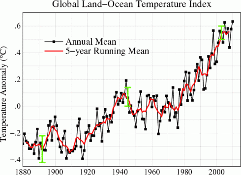
Global Warming: Yes, it’s Warming

Global warming over the last 130 years. The graph shows the temperature anomaly, which is the difference in temperature from the average (0 on the graph). The total change from the 1820's is about 0.8 degrees Celsius. Graph from NASA GISS.

NASA’s Goddard Institute for Space Science has an excellent page that is updated every month, which shows graphs of global temperature changes.

IN addition to the global graphs, there are a lot of really neat graphs showing:

  • separate graphs from the tropics versus the northern hemisphere versus the southern hemisphere (the different latitude bands);
  • the difference between the northern and southern hemispheres;
  • the U.S. only;
  • seasonal changes.

The graphs typically show the temperature anomaly, which is the difference in temperature from the normal. The “normal” is taken to be the average temperature between 1951 and 1980.

Exercise on Wealth Distribution

Using the actual U.S. wealth distribution data from Norton and Arieli (2011; pdf), I created a little addendum to our exercise on the distribution of wealth.

I started with the definition of wealth. Students tend to think you’re referring to annual income, so I gave the example of someone who does not have a job but owns a house; they have no income but some wealth in the value of the house. Alternately, someone who has $2 million in the bank, but owes $4 million, actually has negative wealth.

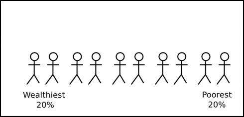
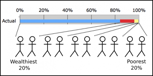
Then I drew a little stick figure diagram to represent the population of the United States. With ten figures, paired up, that gives five parts, aka quintiles.

Breaking the population of the U.S. into five parts (quintiles) based on wealth. The least wealthy are to the right and the most wealthy are to the left.

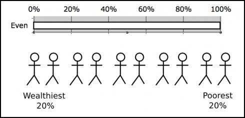
Students were then presented with an empty bar graph and asked, “How much of the U.S.’s wealth is owned by the wealthiest 20% of the population?” Instead of asking in percentages (as are shown in the graph), I asked them to assume that the total wealth in the U.S. is $100 trillion.

Population with empty bar graph.

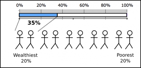
The first suggestion was $35 trillion, which is shown below. Others offered different amounts, ranging up to $50 trillion. Someone even suggested $15 trillion, which is not possible, since that would mean that the wealthiest 20% have less than 20% of the total wealth of the country.

If the wealthiest 20% owned 35% of the wealth of the U.S. the graph would look like this.

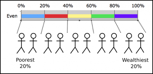
Once they got the idea, I showed them what the graph would look like in an idealized socialist country, where everyone had the same wealth.

An even (socialist) distribution of wealth.

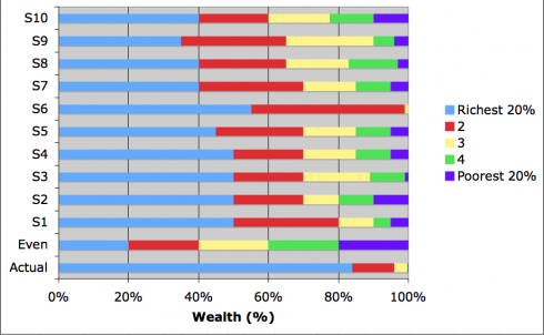
Finally, I asked my students to fill in what they believed to be the actual case for the U.S. for all five quintiles. The results had to add up to $100 trillion. They gave me their numbers individually before we broke up our meeting, and I entered it in the U.S. distribution of wealth spreadsheet to produce a graph.

After lunch, I showed them the results.

Students' beliefs about the distribution of wealth in the U.S. (S1 through S10 and the average student response), compared to an equal distribution and the actual distribution (bottom).

For dramatic effect, I hid the last two bars at first. We talked over their numbers, then I showed them the equal distribution case (which they’d seen before), and finally the actual distribution.

Actual U.S. distribution of wealth. Data from Holder and Arieli (2011)

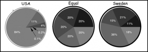
The response was salutary; a moment of surprised silence and then whispers. What then followed was a nice, short discussion. I pointed out the pie charts showing the U.S. versus an equal distribution, versus Sweden and asked what they would do, if they were an autocratic monarch, or if they were the president to make the U.S.’s distribution more equal.

How wealth is shared in the U.S. compared to and equal distribution (middle), compared to Sweden. Image adapted from Norton and Aireli (2011).

We talked about the government just taking private property, like the communists did. Then we talked about progressive taxation. We ended by talking about the estate tax, and meritocracy, which we’d touched on in the morning.

I thought the exercise worked very well. Not only did we get into an interesting economic issue, but got some practice with math and interpreting graphs too.

Distribution of Wealth

One of our economics assignments this cycle asks students to divvy up $200,000 among a group of ten people. One is a divorced mom, another a playboy, a third a bank manager, you get the gist. The purpose is to compare what students think it should be, to what a socialist might believe, to students’ estimation of reality. I’m really curious to see what they come up with.

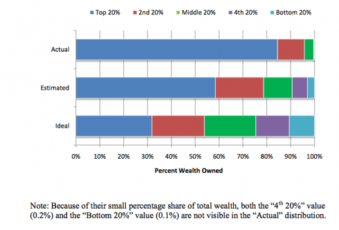
Michael Norton and Dan Ariely have some actual data on the wealth distribution in the United States that might really challenge some assumptions (Norton and Ariely, 2011 pdf). They asked survey respondents what percentage of wealth they thought was owned by the poorest 20% of U.S. citizens, the next 20% and so on. They also asked what kind of wealth distribution people though would be ideal. Finally, they compared what people thought to what was actually there.

The actual distribution of wealth in the U.S. (top), what people think is the case (middle), and people's ideal distribution (bottom). Figure from Norton and Ariely (2011).

People, apparently, really underestimate the income inequality in the U.S..

A second part of the same study gave people pie charts of wealth distribution in different societies and asked them to pick out which one they would prefer to live in if they were dropped at random into one of these societies. They compared the more socialist-like Sweden, to the U.S., and to a perfectly even distribution. People greatly preferred societies with a more equal sharing of wealth.

How wealth is shared in the U.S. compared to and equal distribution (middle), compared to Sweden. Image adapted from Norton and Aireli (2011).

I think I’m going to have to modify this assignment to use these graphs. I’ll also have to use their definition of wealth:

Wealth, also known as net worth, is defined as the total value of everything someone owns minus any debt that he or she owes. A person’s net worth includes his or her bank account savings plus the value of other things such as property, stocks, bonds, art, collections, etc., minus the value of things like loans and mortgages.

–Norton and Arieli (2011): Building a Better America – One Wealth Quintile at a Time in Perspectives on Psychological Science

Graphing discussion threads

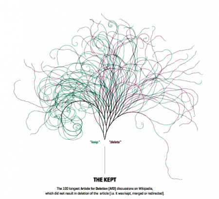
Graphic representation of the Wikipedia discussions about deleting articles. The image links to an interactive version of the graphic at http://notabilia.net .

Swings to the right are arguments for keeping the article, swings to the left are arguments to delete them. Moritz Stefaner and others’ website have created this wonderful graphic of Wikipedia’s discussion threads. They have lots more details and discussions on their website.

“The only time anyone fails is when they are scared to try”

“[My father] used to say it was better to fail through lack of ability than lack of effort,” he says. “He also said fear of failure was something you had to go through because the only time anyone fails is when they are scared to try.”
— Ian Holloway in The Guardian

One of the things I really like about European (and other) soccer leagues is the relegation and promotion system. It encourages competition, and the dream that one day your small town side can make it up the the big leagues. Or as in Blackpool’s case, return to the top after thirty years in the lower divisions.

When they barely qualified for the top English division last year, it was widely expected that they would set records for most goals conceded, and be the first team to be relegated. But they’ve done well enough. They’re well out of the relegation zone at the moment and have impressed, even though they’re still playing in the smallest stadium and have the cheapest team. So their coach, Ian Holloway, knows something about facing potential embarrassment, and the fear of failure.

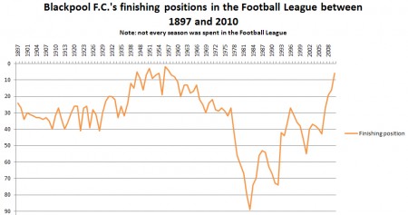
Keeping with our theme of graphing for this cycle, here is a graph showing the position of Blackpool in the English football leagues. Each league has about 20 teams so the graph shows a range of about four divisions. (From Wikipedia user Dudesleeper).

U.S. Immigration Data

Raymond Cohn has a great table of immigration data on the Economic History Association website.

This data ties very nicely into the work we’re doing on graphing. The Excel file with the post 1820 data, and another with pre-1790 data, make it easier to work with (note the pre-1970 data comes from the Wikipedia page on the history of immigration; it was the easiest source to find a table of data).

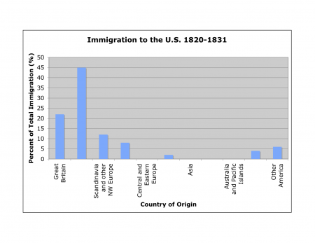
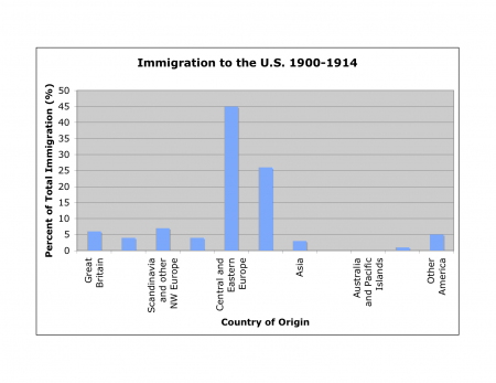
Since each small group of students is responsible for a different wave of immigration, the groups will create bar graphs showing the countries of origin for each wave. They should look like these:

U.S. Immigration from 1820 to 1831. Data from Cohn (2010).

and,

U.S. Immigration from 1900 to 1914. Data from Cohn (2010).

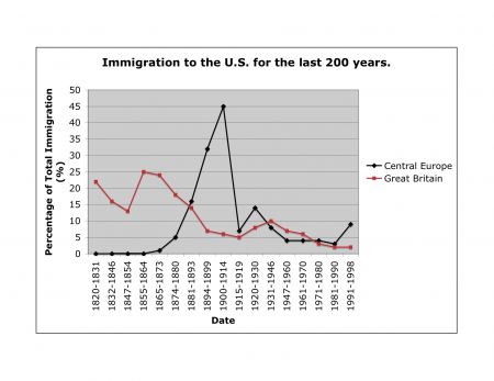
Plotting the time series as a line graph would be another great way to slice the data:

Comparison of U.S. Immigration Rates from Great Britain and Central Europe. Data from Cohn (2010).

Note that the data in the table is as a percentage of total immigration, so the numbers do not compare directly from one time period to the next; however, the proportions still work to show the same patterns.