Following up on the project to find the volume (and surface area) of a guitar, and the slope at a point along the outline of the guitar, I asked students to use the same techniques to estimate the area under a curve (y = x2) and find the slope at a point along the curve. Specifically:
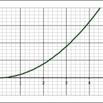
- Draw the function y = x2
- Find the area bounded by the function, the lines x = 1 and x = 4, and the x-axis
- Find the slope of a tangent to the y = x2 function at the point where x = 3.
The point of the second question is to test if students have internalized the idea that they can approximate curved shapes with trapezoids, but they have to weigh the time it will take to do a lot of trapezoids, versus the reduction in error that will result from more trapezoids. It’s interesting to see students’ character come through in this assignment: some choose to make one big trapezoid and are done, while other will go so many trapezoids that they run out of time to get them done.
It just occurs to me, however, that an interesting way to assess this assignment would be to give them a fixed time, and tell them that their score will be the 100 minus the percent error in their calculations.
Limits
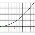
The third question–about finding the slope of a tangent line at x = 3–is our jumping off point into the mathematics of limits and calculus.
Some students do a single approximation–either forward or backward–, while others do both and take the average.
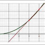
The forward approximation involves finding the values for the function y = x2 at x = 3 and x = 4 and finding the slope between the two points:
- when x = 3, y = 9, so we have the point (x1,y1) = (3, 9)
- when x = 4, y = 16, so we have the point (x2,y2) = (3, 16)
The slope (m) between two points is found with the equation they learned back in algebra:
![]()
Where Δx = x2-x1 and Δy = y2-y1.
Using the two points above gives:
![]()
Those who use the backward approximation simply use the point when x = 2 instead of x = 4, and they end up with a value for the slope of 5.
Averaging the forward and backward approximations give a slope of 6.
Now, since they know that the closer you make the points the better the approximation, I ask them to make a table to see what happens as they do so. This means reducing the value of Δx. In both the forward and backward approximation shown above, Δx = 1.
This can be done very quickly in Excel (or any other spreadsheet program), however, this time at least, most students chose to do it by hand. They end up with a table that looks like this:
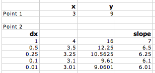

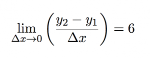
As you plot slope versus the change in x (Δx), you can see that as Δx gets smaller and smaller and approaches zero, the slope gets closer and closer to 6. So we could say that:
the limit of the slope as Δx approaches zero is 6.
Mathematically this can be written as:
or using the equation for slope:
Now, we can work on taking the limit in a more general way to do differentiation.


