Maximum Range of a Potato Gun

One of the middle schoolers built a potato gun for his math class. He was looking a the mathematical relationship between the amount of fuel (hair spray) and the hang-time of the potato. To augment this work, I had my Numerical Methods class do the math and create analytical and numerical models of the projectile motion.

One of the things my students had to figure out was what angle would give the maximum range of the projectile? You can figure this out analytically by finding the function for how the horizontal distance (x) changes as the angle (theta) changes (i.e. x(theta)) and then finding the maximum of the function.

Initial velocity vector (v) and its component vectors in the x and y directions. — Initial velocity vector (v) and its component vectors in the x and y directions for a given angle.

Distance as a function of the angle

In a nutshell, to find the distance traveled by the potato we break its initial velocity into its x and y components (v_x and v_y), use the y component to find the flight time of the projectile (t_f), and then use the v_x component to find the distance traveled over the flight time.

Starting with the diagram above we can separate the initial velocity of the potato into its two components using basic trigonometry:

$\cos{\theta} = \frac{v_x}{v}$
$\sin{\theta} = \frac{v_y}{v}$ ,

so,

$v_x = v \cos{\theta}$ ,
$v_y = v \sin{\theta}$

Now we know that the height of a projectile (y) is given by the function:

$! y(t) = \frac{a t^2}{2} + v_0 t + y_0$

(you can figure this out by assuming that the acceleration due to gravity (a) is constant and acceleration is the second differential of position with respect to time.)

To find the flight time we assume we’re starting with an initial height of zero (y₀ = 0), and that the flight ends when the potato hits the ground which is also at zero ((y_t = 0), so:

$! 0 = \frac{a t^2}{2} + v_0 t + 0$

$! 0 = \frac{a t^2}{2} + v_0 t$

Factoring out t gives:

$! 0 = t ( \frac{a t}{2} + v_0)$

Looking at the two factors, we can now see that there are two solutions to this problem, which should not be too much of a surprise since the height equation is parabolic (a second order polynomial). The solutions are when:

$! t = 0$

$! \frac{a t}{2} + v_0 = 0$

The first solution is obviously the initial launch time, while the second is going to be the flight time (t_f).

$! \frac{a t_f}{2} + v_0 = 0$

$! t_f = - \frac{2 v_0}{a}$

You might think it’s odd to have a negative in the equation, but remember, the acceleration is negative so it’ll cancel out.

Now since we’re working with the y component of the velocity vector, the initial velocity in this equation (v₀) is really just v_y:

$! v_0 = v_y$

so we can substitute in the trig function for v_y to get:

$! t_f = - \frac{2 v \sin{\theta}}{a}$

Our horizontal distance is simply given by the velocity in the x direction (v_x) times the flight time:

$! x = v_x t_f$

which becomes:

$! x = v_x \left(- \frac{2 v \sin{\theta}}{a}\right)$

and substituting in the trig function for v_x (just to make things look more complicated):

$! x = \left( v \cos{\theta} \right) \left(- \frac{2 v \sin{\theta}}{a}\right)$

and factoring out some of the constants gives:

$! x = -\frac{v^2}{a} 2 \sin{\theta}\cos{theta}$

Now we have distance as a function of the launch angle.

We can simplify this a little by using the double-angle formula:

$! \sin{2\theta} = 2 \sin{\theta}\cos{theta}$

to get:

$! x = -\frac{v^2}{a} \sin{2\theta}$

Finding the maximum distance

How do we find the maxima for this function. Sketching the curve should be easy enough, but because we know a little calculus we know that the maximum will occur when the first differential is equal to zero. So we differentiate with respect to the angle to get:

$! \frac{dx}{d\theta} = -\frac{v^2}{a} 2 \cos{2\theta}$

and set the differential equal to zero:

$! 0 = -\frac{v^2}{a} 2 \cos{2\theta}$

and solve to get:

$! \cos{2\theta} = 0$

$! 2\theta = \cos^{-1}{(0)}$

Since we remember that the arccosine of 0 is 90 degrees:

$! 2\theta = 90^{\circ}$

$! \theta = 45^{\circ}$

And thus we’ve found the angle that gives the maximum launch distance for a potato gun.

Basic JavaScript

Basic Webpage template (using Jquery): basic-jquery.zip

One of my students couldn’t get VPython to install and run her computer. She was running Windows 8, and I have not used Windows, much less this version of it to figure out what the problem was. This is one of the challenges with a bring your own device policy. So, instead I gave the lesson on numerical integration using javascript.

To make things easier, I create a barebones template of a webpage build around javascript (using the jquery library to make interactivity easier).

If you open the webpage file (index.html) in your browser you should see nothing but the word “Hello”. The template is blank, but it’s ready so students can start with the javascript programming right away, which a few of my programming elective students have done.

For reference, this file (basic-jquery-numeric-int.zip) uses the template to create a program that does numerical integration. Someone using the webpage can enter the limits (a and b) and the number of trapezoids to use (n), and the program calculates calculates the area under the curve f(x) = -x²/4 + x + 4.

It’s a very bare template and doesn’t have any comments, so it’s not useful unless you’re at least a little familiar with html and javascript and just need a clean place to start.

Programming Numerical Integration with Python (and Javascript)

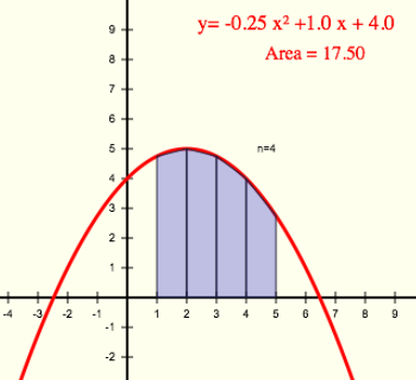
num-int-n4 — Numerically integrating the area under the curve using four trapezoids.

I gave a quick introduction to programming for my calculus class, which has been working on numerical integration.

Numerical integration is usually used for functions that can’t be integrated (or not easily integrated) but for this example we’ll use a simple parabolic function so we can compare the numerical results to the analytical solution (as seen here).

With the equation:

$f(x) = -\frac{1}{4} x^2 + x + 4$

To find the area under the curve between x = 1 and x = 5 we’d find the definite integral:

$Area = \int_{_1}^{^5} \left(-\frac{x^2}{4} + x + 4 \right) \,dx$

which gives the result:

$Area = 17 \frac{2}{3} = 17.6\bar{6}$

For numerical integration, we break the area of concern into a number of trapezoids, find the areas of all the trapezoids and add them up.

We’ll define the left and right boundaries of the area as a and b, and we can write the integral as:

$Area = \int_{_a}^{^b} f(x) \,dx$

num_int-1 — The left and right boundaries of the area we’re interested in are defined as a and b respectively. The area of each trapezoid is defined as A_n.

We also have to choose a number of trapezoids (n) or the width of each trapezoid (dx). Here we choose four trapezoids (n = 4), which gives a trapezoid width of one (dx = 1).

num_int-2 — The area of the first trapezoid can be calculated from its width (dx) and the height of the two upper ends of the trapezoid (f(x₀) and f(x₁).

So if we define the x values of the left and right sides of the first trapezoids as x₀ and x₁, the area of the first trapezoid is:

$A_1 = \frac{f(x_{_0})+f(x_{_1})}{2} dx$

For this program, we’ll set the trapezoid width (dx) and then calculate the number of trapezoids (n) based on the width and the locations of the end boundaries a and b. So:

$n = \frac{b-a}{dx}$

and the sum of all the areas will be:

$\displaystyle\sum\limits_{i=1}^{n} \frac{f(x_{i-1})+f(x_{i})}{2} dx$

We can also figure out that since the x values change by the same value (dx) for every trapezoid, it’s an arithmetic progression, so:

$x_{i-1} = a + (i-1) dx$

and,

$x_{i} = a + i \cdot dx$

so our summation becomes:

$\displaystyle\sum\limits_{i=1}^{n} \frac{f(a+(i-1)dx)+f(a + i \cdot dx)}{2} dx$

Which we can program with:

numerical_integration.py

# the function to be integrated
def func(x):
    return -0.25*x**2 + x + 4

# define variables
a = 1.          # left boundary of area
b = 5.          # right boundary of area
dx = 1          # width of the trapezoids

# calculate the number of trapezoids
n = int((b - a) / dx)

# define the variable for area
Area = 0

# loop to calculate the area of each trapezoid and sum.
for i in range(1, n+1):
    #the x locations of the left and right side of each trapezpoid
    x0 = a+(i-1)*dx
    x1 = a+i*dx

    #the area of each trapezoid
    Ai = dx * (func(x0) + func(x1))/ 2.

    # cumulatively sum the areas
    Area = Area + Ai

#print out the result.
print "Area = ", Area

And the output looks like

>>> 
Area =  17.5
>>>

While the programming is pretty straightforward, it was a bit of a pain getting Python to work for one of my students who is running Windows 8. I still have not figured out a way to get it to work properly, so I’m considering trying to do it using Javascript.

Update

The javascript functions for numerical integration:

function numerically_integrate(a, b, dx, f) {
	
	// calculate the number of trapezoids
	n = (b - a) / dx;
	
	// define the variable for area
	Area = 0;
	
	//loop to calculate the area of each trapezoid and sum.
	for (i = 1; i <= n; i++) {
		//the x locations of the left and right side of each trapezpoid
		x0 = a + (i-1)*dx;
		x1 = a + i*dx;
		
		// the area of each trapezoid
		Ai = dx * (f(x0) + f(x1))/ 2.;
		
		// cumulatively sum the areas
		Area = Area + Ai	
		
	} 
	return Area;
}

//define function to be integrated
function f(x){
	return -0.25*Math.pow(x,2) + x + 4;
}

// define variables
a = 1;		// left boundary of area
b = 5;		// right boundary of area
dx = 1;		// width of the trapezoids
	
// print out output
alert("Area = "+ numerically_integrate(a, b, dx, f));

This is a demonstration of a full html file that uses the function, and should work in any modern browser (download files: numerical-integration.zip).

Update 2

I’ve added the above javascript code to the embeddable graphs to allow it to calculate and display numerical integrals: you can change the values in the interactive graph below.

Exponential Cell Growth

The video shows 300 seconds of purely exponential growth (uninhibited), captured from the exponential growth VAMP scenario. Like the exponential growth function itself, the video starts off slowly then gets a lot more exciting (for a given value of exciting).

The modeled growth is based on the exponential growth function:

$N = N_0 e^{rt}$ (1)

where:

N = number of cells (or concentration of biomass);
N₀ = the starting number of cells;
r = the rate constant, which determines how fast growth occurs; and
t = time.

Finding the Rate Constant/Doubling Time (r)

You can enter either the rate constant (r) or the doubling time of the particular organism into the model. Determining the doubling time from the exponential growth equation is a nice exercise for pre-calculus students.

Let’s call the doubling time, t_d. When the organism doubles from it’s initial concentration the growth equation becomes:

$2N_0 = N_0 e^{r t_d}$

divide through by N₀:

$2 = e^{r t_d}$

take the natural logs of both sides:

$\ln 2 = \ln (e^{r t_d})$

bring the exponent down (that’s one of the rules of logarithms);

$\ln 2 = r t_d \ln (e)$

remember that ln(e) = 1:

$\ln 2 = r t_d$

and solve for the doubling time:

$\frac{\ln 2}{r} = t_d$

Decay

A nice follow up would be to solve for the half life given the exponential decay function, which differs from the exponential growth function only by the negative in the exponent:

$N = N_0 e^{-rt}$

The UCSD math website has more details about Exponential Growth and Decay.

Finding the Growth Rate

A useful calculus assignment would be to determine the growth rate at any point in time, because that’s what the model actually uses to calculate the growth in cells from timestep to timestep.

The growth rate would be the change in the number of cells with time:

$\frac{dN}{dt}$

starting with the exponential growth equation:

$N = N_0 e^{rt}$

since we have a natural exponent term, we’ll use the rule for differentiating natural exponents:

$\frac{d}{dx}(e^u) = e^u \frac{du}{dx}$

So to make this work we’ll have to define:

$u = rt$

which can be differentiated to give:

$\frac{du}{dt} = r$

and since N₀ is a constant:

$N = N_0 e^{u}$

$\frac{dN}{dt} = N_0 e^{u} \frac{du}{dt}$

substituting in for u and du/dt gives:

$\frac{dN}{dt} = N_0 e^{rt} (r)$

rearranging (to make it look prettier (and clearer)):

$\frac{dN}{dt} = N_0 r e^{rt}$ (2)

Numerical Methods: Euler’s method

With this formula, the model could use linear approximations — like in Euler’s method — to simulate the growth of the biomass.

First we can discretize the differential so that the change in N and the change in time (t$) take on discrete values:
$\frac{dN}{dt} = \frac{\Delta N}{\Delta t}$

Now the change in N is the difference between the current value N^t and the new value N^t+1:

Now using this in our differentiated equation (Eq. 2) gives:

$\frac{N^{t+1}-N^t}{\Delta t} = N_0 r e^{r\Delta t}$

Which we can solve for the new biomass (N^^t+1):

$N^{t+1}-N^t = N_0 r e^{r\Delta t} \Delta t$

to get:
$N^{t+1} = N_0 r e^{r\Delta t} \Delta t + N^t$

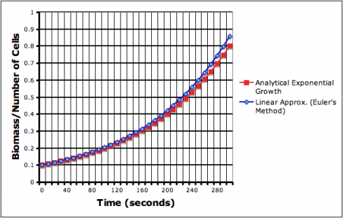
This linear approximation, however, does introduce some error.

The approximated exponential growth curve (blue line) deviates from the analytical equation. The deviation compounds itself, getting worse exponentially, as time goes on.

Excel file for graphed data: exponential_growth.xls

VAMP

This is the first, basic but useful product of my summer work on the IMPS website, which is centered on the VAMP biochemical model. The VAMP model is, as of this moment, still in it’s alpha stage of development — it’s not terribly user-friendly and is fairly limited in scope — but is improving rapidly.

Learning Matricies by Programming a Matrix Solver

One of my pre-Calculus students convinced me that the best way for him to learn how to work with matrices was for him to program a matrix solver. I helped him create a Gaussian Elimination solver in Python (which we’ve been using since last year).

Gaussian Elimination Matrix Solver by Alex Shine (comments by me).

from visual import *

'''The coefficient matrix (m) can be any sized square matrix 
   with an additional column for the solution'''
m = [ [1,-2,1,-4],[0,1,2,4],[2,3,-2,2]]

'''Convert the input matrix, m (which is a list) into an array'''
a = array(m,float)
print "Input matrix:"
print a
print

'''Get the shape of the matrix (number of rows and columns)'''
(r,c) = a.shape 

rs = (1-r)

'''Solve'''
for j in range(r):

    print "Column #:", j
    for i in range(r):
        if a[i,j] <> 0:
            a[i,:] = a[i,:] / a[i,j]
    print a
    print

    for i in range(rs+j,j):
        if a[i,j] <> 0:
            a[i,:] = a[j,:] - a[i,:]
    print a
    print

print "Solution"
for i in range (r):
    a[i,:] = a[i,:] / a[i,i]
    print "Variable", i, "=", a[i,-1]

print
print "Solution Matrix:"
print a

The code above solves the following system of equations:


  x - 2y +  z = -4 
       y + 2z =  4 
 2x + 3y - 2z =  2

Which can be written in matrix form as such:

$\left[ \begin{array}{ccc} 1 & -2 & 1 \\ 0 & 1 & 2 \\ 2 & 3 & -2 \end{array} \right] \left[ \begin{array}{c} x \\ y \\ z \end{array} \right] = \left[ \begin{array}{c} -4 \\ 4 \\ 2 \end{array} \right]$

You use the solver by taking the square matrix on the left hand side of the equation and combining it with the column on the hand side as an additional column:

$\left[ \begin{array}{cccc} 1 & -2 & 1 & -4 \\ 0 & 1 & 2 & 4\\ 2 & 3 & -2 & 2\end{array} \right]$

This is entered into the program as the line:

m = [ [1,-2,1,-4],[0,1,2,4],[2,3,-2,2]]

When you run the above program you should get the results:

>>> ================================ RESTART ================================
>>> 
Input matrix:
[[ 1. -2.  1. -4.]
 [ 0.  1.  2.  4.]
 [ 2.  3. -2.  2.]]

Column #: 0
[[ 1.  -2.   1.  -4. ]
 [ 0.   1.   2.   4. ]
 [ 1.   1.5 -1.   1. ]]

[[ 1.  -2.   1.  -4. ]
 [ 0.   1.   2.   4. ]
 [ 0.  -3.5  2.  -5. ]]

Column #: 1
[[-0.5         1.         -0.5         2.        ]
 [ 0.          1.          2.          4.        ]
 [-0.          1.         -0.57142857  1.42857143]]

[[ 0.5         0.          2.5         2.        ]
 [ 0.          1.          2.          4.        ]
 [ 0.          0.          2.57142857  2.57142857]]

Column #: 2
[[ 0.2  0.   1.   0.8]
 [ 0.   0.5  1.   2. ]
 [ 0.   0.   1.   1. ]]

[[-0.2  0.   0.   0.2]
 [ 0.  -0.5  0.  -1. ]
 [ 0.   0.   1.   1. ]]

Solution
Variable 0 = -1.0
Variable 1 = 2.0
Variable 2 = 1.0

Solution Matrix:
[[ 1. -0. -0. -1.]
 [-0.  1. -0.  2.]
 [ 0.  0.  1.  1.]]
>>>

Be aware that:

The code is designed to take any size of matrix.
The matrix you put in can not have any zeros on its diagonal, so some manipulation is often necessary before you can use the code.

Other notes:

The negative zeros (-0) that show up especially in the solution matrix may not look pretty but do not affect the solution.
The code imports the vpython module in the first line but what it really needs is the numpy module, which vpython imports, for the arrays.

The next step is to turn this into a function or a class that can be used in other codes, but it’s already proved useful. My calculus students compared their solutions for the coefficients of a quadratic equation that they had to solve for their carpet friction experiment, which was great because their first answers were wrong.