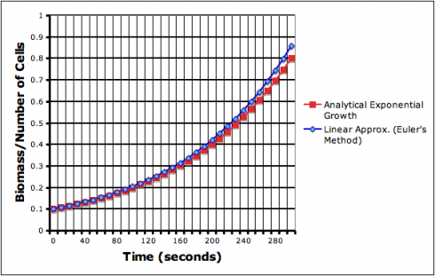
The video shows 300 seconds of purely exponential growth (uninhibited), captured from the exponential growth VAMP scenario. Like the exponential growth function itself, the video starts off slowly then gets a lot more exciting (for a given value of exciting).
The modeled growth is based on the exponential growth function:
![]() (1)
(1)
where:
- N = number of cells (or concentration of biomass);
- N0 = the starting number of cells;
- r = the rate constant, which determines how fast growth occurs; and
- t = time.
Finding the Rate Constant/Doubling Time (r)
You can enter either the rate constant (r) or the doubling time of the particular organism into the model. Determining the doubling time from the exponential growth equation is a nice exercise for pre-calculus students.
Let’s call the doubling time, td. When the organism doubles from it’s initial concentration the growth equation becomes:
![]()
divide through by N0:
![]()
take the natural logs of both sides:
![]()
bring the exponent down (that’s one of the rules of logarithms);
![]()
remember that ln(e) = 1:
![]()
and solve for the doubling time:
![]()
Decay
A nice follow up would be to solve for the half life given the exponential decay function, which differs from the exponential growth function only by the negative in the exponent:
![]()
The UCSD math website has more details about Exponential Growth and Decay.
Finding the Growth Rate
A useful calculus assignment would be to determine the growth rate at any point in time, because that’s what the model actually uses to calculate the growth in cells from timestep to timestep.
The growth rate would be the change in the number of cells with time:
![]()
starting with the exponential growth equation:
![]()
since we have a natural exponent term, we’ll use the rule for differentiating natural exponents:
![]()
So to make this work we’ll have to define:
![]()
which can be differentiated to give:
![]()
and since N0 is a constant:
![]()
![]()
substituting in for u and du/dt gives:
![]()
rearranging (to make it look prettier (and clearer)):
![]() (2)
(2)
Numerical Methods: Euler’s method
With this formula, the model could use linear approximations — like in Euler’s method — to simulate the growth of the biomass.
First we can discretize the differential so that the change in N and the change in time (t$) take on discrete values:
![]()
Now the change in N is the difference between the current value Nt and the new value Nt+1:
Now using this in our differentiated equation (Eq. 2) gives:
![]()
Which we can solve for the new biomass (N^t+1):
![]()
to get:
![]()
This linear approximation, however, does introduce some error.

Excel file for graphed data: exponential_growth.xls
VAMP
This is the first, basic but useful product of my summer work on the IMPS website, which is centered on the VAMP biochemical model. The VAMP model is, as of this moment, still in it’s alpha stage of development — it’s not terribly user-friendly and is fairly limited in scope — but is improving rapidly.