Programming Numerical Integration with Python (and Javascript)

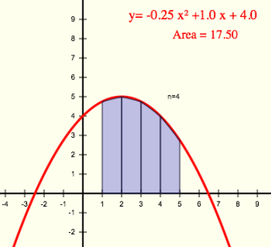
num-int-n4 — Numerically integrating the area under the curve using four trapezoids.

I gave a quick introduction to programming for my calculus class, which has been working on numerical integration.

Numerical integration is usually used for functions that can’t be integrated (or not easily integrated) but for this example we’ll use a simple parabolic function so we can compare the numerical results to the analytical solution (as seen here).

With the equation:

$f(x) = -\frac{1}{4} x^2 + x + 4$

To find the area under the curve between x = 1 and x = 5 we’d find the definite integral:

$Area = \int_{_1}^{^5} \left(-\frac{x^2}{4} + x + 4 \right) \,dx$

which gives the result:

$Area = 17 \frac{2}{3} = 17.6\bar{6}$

For numerical integration, we break the area of concern into a number of trapezoids, find the areas of all the trapezoids and add them up.

We’ll define the left and right boundaries of the area as a and b, and we can write the integral as:

$Area = \int_{_a}^{^b} f(x) \,dx$

num_int-1 — The left and right boundaries of the area we’re interested in are defined as a and b respectively. The area of each trapezoid is defined as A_n.

We also have to choose a number of trapezoids (n) or the width of each trapezoid (dx). Here we choose four trapezoids (n = 4), which gives a trapezoid width of one (dx = 1).

num_int-2 — The area of the first trapezoid can be calculated from its width (dx) and the height of the two upper ends of the trapezoid (f(x₀) and f(x₁).

So if we define the x values of the left and right sides of the first trapezoids as x₀ and x₁, the area of the first trapezoid is:

$A_1 = \frac{f(x_{_0})+f(x_{_1})}{2} dx$

For this program, we’ll set the trapezoid width (dx) and then calculate the number of trapezoids (n) based on the width and the locations of the end boundaries a and b. So:

$n = \frac{b-a}{dx}$

and the sum of all the areas will be:

$\displaystyle\sum\limits_{i=1}^{n} \frac{f(x_{i-1})+f(x_{i})}{2} dx$

We can also figure out that since the x values change by the same value (dx) for every trapezoid, it’s an arithmetic progression, so:

$x_{i-1} = a + (i-1) dx$

and,

$x_{i} = a + i \cdot dx$

so our summation becomes:

$\displaystyle\sum\limits_{i=1}^{n} \frac{f(a+(i-1)dx)+f(a + i \cdot dx)}{2} dx$

Which we can program with:

numerical_integration.py

# the function to be integrated
def func(x):
    return -0.25*x**2 + x + 4

# define variables
a = 1.          # left boundary of area
b = 5.          # right boundary of area
dx = 1          # width of the trapezoids

# calculate the number of trapezoids
n = int((b - a) / dx)

# define the variable for area
Area = 0

# loop to calculate the area of each trapezoid and sum.
for i in range(1, n+1):
    #the x locations of the left and right side of each trapezpoid
    x0 = a+(i-1)*dx
    x1 = a+i*dx

    #the area of each trapezoid
    Ai = dx * (func(x0) + func(x1))/ 2.

    # cumulatively sum the areas
    Area = Area + Ai

#print out the result.
print "Area = ", Area

And the output looks like

>>> 
Area =  17.5
>>>

While the programming is pretty straightforward, it was a bit of a pain getting Python to work for one of my students who is running Windows 8. I still have not figured out a way to get it to work properly, so I’m considering trying to do it using Javascript.

Update

The javascript functions for numerical integration:

function numerically_integrate(a, b, dx, f) {
	
	// calculate the number of trapezoids
	n = (b - a) / dx;
	
	// define the variable for area
	Area = 0;
	
	//loop to calculate the area of each trapezoid and sum.
	for (i = 1; i <= n; i++) {
		//the x locations of the left and right side of each trapezpoid
		x0 = a + (i-1)*dx;
		x1 = a + i*dx;
		
		// the area of each trapezoid
		Ai = dx * (f(x0) + f(x1))/ 2.;
		
		// cumulatively sum the areas
		Area = Area + Ai	
		
	} 
	return Area;
}

//define function to be integrated
function f(x){
	return -0.25*Math.pow(x,2) + x + 4;
}

// define variables
a = 1;		// left boundary of area
b = 5;		// right boundary of area
dx = 1;		// width of the trapezoids
	
// print out output
alert("Area = "+ numerically_integrate(a, b, dx, f));

This is a demonstration of a full html file that uses the function, and should work in any modern browser (download files: numerical-integration.zip).

Update 2

I’ve added the above javascript code to the embeddable graphs to allow it to calculate and display numerical integrals: you can change the values in the interactive graph below.

Exponential Cell Growth

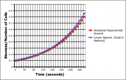
The video shows 300 seconds of purely exponential growth (uninhibited), captured from the exponential growth VAMP scenario. Like the exponential growth function itself, the video starts off slowly then gets a lot more exciting (for a given value of exciting).

The modeled growth is based on the exponential growth function:

$N = N_0 e^{rt}$ (1)

where:

N = number of cells (or concentration of biomass);
N₀ = the starting number of cells;
r = the rate constant, which determines how fast growth occurs; and
t = time.

Finding the Rate Constant/Doubling Time (r)

You can enter either the rate constant (r) or the doubling time of the particular organism into the model. Determining the doubling time from the exponential growth equation is a nice exercise for pre-calculus students.

Let’s call the doubling time, t_d. When the organism doubles from it’s initial concentration the growth equation becomes:

$2N_0 = N_0 e^{r t_d}$

divide through by N₀:

$2 = e^{r t_d}$

take the natural logs of both sides:

$\ln 2 = \ln (e^{r t_d})$

bring the exponent down (that’s one of the rules of logarithms);

$\ln 2 = r t_d \ln (e)$

remember that ln(e) = 1:

$\ln 2 = r t_d$

and solve for the doubling time:

$\frac{\ln 2}{r} = t_d$

Decay

A nice follow up would be to solve for the half life given the exponential decay function, which differs from the exponential growth function only by the negative in the exponent:

$N = N_0 e^{-rt}$

The UCSD math website has more details about Exponential Growth and Decay.

Finding the Growth Rate

A useful calculus assignment would be to determine the growth rate at any point in time, because that’s what the model actually uses to calculate the growth in cells from timestep to timestep.

The growth rate would be the change in the number of cells with time:

$\frac{dN}{dt}$

starting with the exponential growth equation:

$N = N_0 e^{rt}$

since we have a natural exponent term, we’ll use the rule for differentiating natural exponents:

$\frac{d}{dx}(e^u) = e^u \frac{du}{dx}$

So to make this work we’ll have to define:

$u = rt$

which can be differentiated to give:

$\frac{du}{dt} = r$

and since N₀ is a constant:

$N = N_0 e^{u}$

$\frac{dN}{dt} = N_0 e^{u} \frac{du}{dt}$

substituting in for u and du/dt gives:

$\frac{dN}{dt} = N_0 e^{rt} (r)$

rearranging (to make it look prettier (and clearer)):

$\frac{dN}{dt} = N_0 r e^{rt}$ (2)

Numerical Methods: Euler’s method

With this formula, the model could use linear approximations — like in Euler’s method — to simulate the growth of the biomass.

First we can discretize the differential so that the change in N and the change in time (t$) take on discrete values:
$\frac{dN}{dt} = \frac{\Delta N}{\Delta t}$

Now the change in N is the difference between the current value N^t and the new value N^t+1:

Now using this in our differentiated equation (Eq. 2) gives:

$\frac{N^{t+1}-N^t}{\Delta t} = N_0 r e^{r\Delta t}$

Which we can solve for the new biomass (N^^t+1):

$N^{t+1}-N^t = N_0 r e^{r\Delta t} \Delta t$

to get:
$N^{t+1} = N_0 r e^{r\Delta t} \Delta t + N^t$

This linear approximation, however, does introduce some error.

The approximated exponential growth curve (blue line) deviates from the analytical equation. The deviation compounds itself, getting worse exponentially, as time goes on.

Excel file for graphed data: exponential_growth.xls

VAMP

This is the first, basic but useful product of my summer work on the IMPS website, which is centered on the VAMP biochemical model. The VAMP model is, as of this moment, still in it’s alpha stage of development — it’s not terribly user-friendly and is fairly limited in scope — but is improving rapidly.

Euler’s Method for Approximating a Solution to a Differential Equation

Based on Euler’s Method, this interactive graph illustrates a numerical method for solving differential equations. This approach is at the core of many sophisticated computer models of physical phenomena (like climate and weather).

[inline]

Starting point: (x,y) = ( , )
Step size:
Direction:

Slope equation: dy/dx = x +
Show analytical solution:

If you know the equation for the slope of a curve (the red line for example),

and a point that the curve passes through, such as , you can integrate to find the equation of the curve:

[script type=”text/javascript”]

var width=500;
var height=500;
var xrange=10;
var yrange=10;

mx = width/(2.0*xrange);
bx = width/2.0;
my = -height/(2.0*yrange);
by = height/2.0;

function upause () {
ct = 1;
}

function draw_9110(ctx, polys) {
t_9110=t_9110+dt_9110;
//ctx.fillText (“t=”+t, xp(5), yp(5));
ctx.clearRect(0,0,width,height);

polys[0].drawAxes(ctx);
polys[0].slopeField(ctx, 1.0, 1.0, 0.5);
ctx.lineWidth=2;
polys[0].draw(ctx);
polys[0].write_eqn(ctx, “slope = dy/dx”);

eu = eu_9110;
//override nsteps values
//max_nsteps_9110 = eu.nsteps;
//eu.nsteps = nsteps_9110;

if (nsteps_9110 <= max_nsteps_9110) { nsteps_9110 = nsteps_9110 + 1;} else { nsteps_9110 = 0; } eu.nsteps = nsteps_9110; if (show_parabola_9110 == 1) { polys[0].Integrate(ctx, eu.x1, eu.y1); polys[0].integral.color = '#3c3'; polys[0].integral.draw(ctx); } pos = polys[0].EulerApprox(ctx, eu); //document.getElementById('comment_9110').innerHTML = eu.nsteps+ " " + eu.x1 + " " + eu.y1+ " " + eu.dx+ " " + eu.dir+ " " + max_nsteps_9110; //starting point label ctx.textAlign="right"; ctx.textBaseline="alphabetic"; ctx.font = "14pt Calibri"; ctx.fillStyle = "#00f"; ctx.fillText ('start = ('+eu.x1+','+eu.y1+")", xp(eu.x1-0.25), yp(eu.y1-0.5)); //pos = polys[0].EulerApprox(ctx, st_pt_x_9110, st_pt_y_9110, 0.5,20,-1); //pos = polys[0].EulerApprox(ctx, st_pt_x_9110, st_pt_y_9110, 1, 6,1); //draw starting point ctx.strokeStyle="#00f"; ctx.lineWidth=2; ctx.beginPath(); ctx.arc(xp(eu.x1),yp(eu.y1),dxp(0.1),0,Math.PI*2); ctx.closePath(); ctx.stroke(); //ctx.fillText (' c='+move_dir_9110+' '+polys[1].c, xp(5), yp(5)); } //init_mouse(); var c_9110=document.getElementById("myCanvas_9110"); var ctx_9110=c_9110.getContext("2d"); var change = 0.0001; function create_lines_9110 () { //draw line var polys = []; polys.push(addPoly(0, 0.5, -1)); return polys; } function set_max_nsteps_9110 (eu) { max_nsteps_9110 = 1.5*(xrange - eu.x1)/eu.dx; } var polys_9110 = create_lines_9110(); var x1=xp(-10); var y1=yp(1); var x2=xp(10); var y2=yp(1); var dc_9110=0.05; var t_9110 = 0; var dt_9110 = 500; var st_dx_9110 = 1.0; var st_nsteps_9110 = 0; var nsteps_9110 = 0; var max_nsteps_9110 = 20; var dir_9110 = 1; var show_parabola_9110 = 1; var st_pt_x_9110 = -2; var st_pt_y_9110 = -3; var move_dir_9110 = 1.0; // 1 for up //Form interaction function update_form_9110 (x, y, dx, nsteps, dir, b, c, show_para) { x_9110.value = st_pt_x_9110+""; y_9110.value = st_pt_y_9110+""; dx_9110.value = st_dx_9110.toPrecision(2); //c_max_nsteps_9110.value = max_nsteps_9110+""; //document.getElementById('comment_9110').innerHTML = c_dir_9110; if (dir == 1) { c_dir_9110.selectedIndex = 0; } else {c_dir_9110.selectedIndex = 1;} b_9110.value = b+""; c_9110.value = c+""; if (show_para == 1) { ctrl_show.checked = 1; } else {ctrl_show.checked = 0;} } function get_euler_form_9110 () { pos = {x : parseFloat(x_9110.value), y : parseFloat(y_9110.value)} if (c_dir_9110.selectedIndex == 0) { dir = 1;} else {dir = -1;} eu = addEuler(pos.x, pos.y, parseFloat(dx_9110.value), max_nsteps_9110, dir); return eu } function update_solution_9110 (ctx, eu) { //update equations and solution document.getElementById('slope_eqn_9110').innerHTML = polys_9110[0].get_eqn("dy/dx"); //document.getElementById('eqn_9110').innerHTML = "hey"+eu.y1; polys_9110[0].Integrate(ctx, eu.x1, eu.y1); document.getElementById('eqn_9110').innerHTML = polys_9110[0].integral.get_eqn(); document.getElementById('init_pt_9110').innerHTML = "("+eu.x1+","+eu.y1+")"; } function add_euler_line() { eu_9110 = get_euler_form_9110 (); max_nsteps_9110 = eu_9110.nsteps; nsteps_9110 = 0; } var x_9110 = document.getElementById("x_9110"); var y_9110 = document.getElementById("y_9110"); var dx_9110 = document.getElementById("dx_9110"); //var c_max_nsteps_9110 = document.getElementById("nsteps_9110"); var c_dir_9110 = document.getElementById("dir_9110"); var b_9110 = document.getElementById("b_9110"); var c_9110 = document.getElementById("c_9110"); var ctrl_show = document.getElementById("chk_show_para_9110"); update_form_9110(x_9110, y_9110, dx_9110, nsteps_9110, dir_9110, polys_9110[0].b, polys_9110[0].c, show_parabola_9110); var eu_9110 = get_euler_form_9110 (); set_max_nsteps_9110(eu_9110); update_solution_9110(ctx_9110, eu_9110); setInterval("draw_9110(ctx_9110, polys_9110)", dt_9110); x_9110.onchange = function() { eu_9110 = get_euler_form_9110 (); max_nsteps_9110 = eu_9110.nsteps; nsteps_9110 = 0; } y_9110.onchange = function() { eu_9110 = get_euler_form_9110 (); max_nsteps_9110 = eu_9110.nsteps; nsteps_9110 = 0; } c_dir_9110.onchange = function() { eu_9110 = get_euler_form_9110 (); max_nsteps_9110 = eu_9110.nsteps; nsteps_9110 = 0; } dx_9110.onchange = function() { eu_9110 = get_euler_form_9110 (); max_nsteps_9110 = eu_9110.nsteps; //max_nsteps_9110 = 1.4 * (10 - eu_9110.x1)/eu_9110.dx; set_max_nsteps_9110(eu_9110); nsteps_9110 = 0; } b_9110.onchange = function() { polys_9110[0].set_b(parseFloat(this.value)); eu_9110 = get_euler_form_9110 (); max_nsteps_9110 = eu_9110.nsteps; nsteps_9110 = 0; } c_9110.onchange = function() { polys_9110[0].set_c(parseFloat(this.value)); eu_9110 = get_euler_form_9110 (); max_nsteps_9110 = eu_9110.nsteps; nsteps_9110 = 0; } ctrl_show.onchange = function() { if (this.checked == 1) { show_parabola_9110 = 1;} else {show_parabola_9110 = 0} } [/script] [/inline]

If you don’t have a starting point (initial condition), you can draw a slope field to see what the general pattern of all the possible solutions.

Even with a starting point, however, there are just times when you can’t integrate the slope equation — it’s either too difficult or even impossible.

Then, what you can do is come up with an approximation of what the curve looks like by projecting along the slope from the starting point.

The program above demonstrates how it’s done. This approach is called Euler’s Method, and is gives a numerical approximation rather than finding the exact, analytical solution using calculus (integration).

So why use an approximation when you can find the exact solution? Because, there are quite a number of problems that are impossible or extremely difficult to solve analytically, things like: the diffusion of pollution in a lake; how changing temperature in the atmosphere gives you weather and climate; the flow of groundwater in aquifers; stresses on structural members of buildings; and the list goes on and on.

As with most types of numerical approximations, you get better results if you can reduce the step size between projections of the slope. Try changing the numbers and see.

A more detailed version, with solutions, is here: Euler’s Method.

A good reference: Euler’s Method by Paul Dawkins.

Numerical Integration

This is an attempt to illustrate numerical integration by animating an HTML5’s canvas.

We’re trying to find the area between x = 1 and x = 5, beneath the parabola:

$y = -\frac{1}{4} x^2 + x + 4$

By integrating, the area under the curve can be calculated as being 17 ⅔ (see below for the analytical solution). For numerical integration, however, the area under the curve is filled with trapezoids and the total area is calculated from the sum of all the areas. As you increase the number of trapezoids, the approximation becomes more accurate. The reduction in the error can be seen on the graph: with 1 trapezoid there is a large gap between the shaded area and the curve; more trapezoids fill in the gap better and better.

The table below show how the error (defined as the difference between the calculation using trapezoids and the analytic solution) gets smaller with increasing numbers of trapezoids (n).

Number of trapezoids	Area (units²)	Error (difference from 17.66)
1	15.00	2.66
2	17.00	0.66
3	17.37	0.29
4	17.50	0.16
5	17.56	0.10
6	17.59	0.07
7	17.61	0.05
8	17.63	0.03
9	17.63	0.03
10	17.64	0.02

Analytic solution

The area under the curve, between x = 1 and x = 5 can be figured out analytically by integrating between these limits.

$Area = \int_{_1}^{^5} \left(-\frac{x^2}{4} + x + 4 \right) \,dx$

$Area = \left[-\frac{x^3}{12} + \frac{x^2}{2} + 4x \right]_1^5$

$Area = \left[-\frac{(5)^3}{12} + \frac{(5)^2}{2} + 4(5) \right] - \left[-\frac{(1)^3}{12} + \frac{(1)^2}{2} + 4(1) \right]$

$Area = \left[-\frac{125}{12} + \frac{25}{2} + 16 \right] - \left[-\frac{1}{12} + \frac{1}{2} + 4 \right]$

$Area = \left[ 22 \frac{1}{12} \right] - \left[4 \frac{5}{12} \right]$

$Area = 17 \frac{2}{3} = 17.6\bar{6}$

(See also WolframAlpha’s solution).

Update

Demonstration of this numerical integration using four trapezoids in embeddable graphs.