Embeddable Graphs

Going beyond just polynomials, I’ve created a javascript graphing app that’s easily embeddable.

At the moment, it just does polynomials and points, but polynomials can be used to teach quadratic functions (parabolas) and straight lines to pre-algebra and algebra students. Which I’ve been doing.

Based on my students’ feedback, I’ve made it so that when you change the equation of the line the movement animates. This makes it much easier to see what happens when, for example, you change the slope of a line.

P.S. You can also turn off the interactivity if you just want to show a simple graph. y = x²-1 is shown below:

Introducing Polynomials

If you recall, straight lines have a general equation that looks like this:

$y=mx+b$ (1)

This is called the slope-intercept form of the equation, because m gives the slope, and b tells where the line intercepts the y-axis. For example the line:

$y=2x-3$ (2)

looks like:

Now, in the slope-intercept form, m and b represent numbers. In our example, m = 2 and b = 3.

So what if, instead of calling them m and b we used the same letter (let’s use a) and just gave two different subscripts so:

$m = a_1$ and,
$b = a_0$

therefore equation (1):

$y=mx+b$

becomes:
$y = a_1 x + a_0$ (3)

Now, in case you’re wondering why we picked m = a₁ instead of m = a₀, it’s because of the exponents of x. You see, in the equation x has an exponent of 1, and the constant b could be thought to be multiplying x with an exponent of 0. Considering this, we could rewrite our equation of the line (2):

$y=2x^1-3x^0$ (4)

since:
$x^1 = x$ and,
$x^0 = 1$

we get:
$y=2x-3(1)$
$y=2x-3$

So in equation (3) the subscript refers to the exponent of x.

Now we can expand this a bit more. What if we had a term with x² in an equation:

$y=\frac{1}{2}x^2 + 2x - 3$ (5)

Now we have three coefficients:

$a_0 = -3$ ,
$a_1 = 2$ and,
$a_2 = \frac{1}{2}$ ,

And the graph would look like this.

Because of the x² term (specifically because it has the highest exponent in the equation), this is called a second-order polynomial — that’s why the graph above has a little input box where the order is 2. In fact, on the graph above, you can change the order to see how the equation changes. Indeed, you can also change the coefficients to see how the graph changes.

A second order polynomial is a parabola, while, as you’ve probably guessed, a first order polynomial is a straight line. What’s a zero’th order polynomial?

Finally, we can write a general equation for a polynomial — just like we have the slope-intercept form of a line — using the a coefficients like:

$y = a_n x^n + ... + a_2 x^2 + a_1 x + a_0$

You can use the graphs to tinker around and see what different order polynomials look like, and how changing the coefficients change the graphs. I sort-of like the one below:

References

WolframAlpha has more details on polynomials.

The embedded graphs come from my own Polynomial Grapher.

Euler’s Method for Approximating a Solution to a Differential Equation

Based on Euler’s Method, this interactive graph illustrates a numerical method for solving differential equations. This approach is at the core of many sophisticated computer models of physical phenomena (like climate and weather).

[inline]

Starting point: (x,y) = ( , )
Step size:
Direction:

Slope equation: dy/dx = x +
Show analytical solution:

If you know the equation for the slope of a curve (the red line for example),

and a point that the curve passes through, such as , you can integrate to find the equation of the curve:

[script type=”text/javascript”]

var width=500;
var height=500;
var xrange=10;
var yrange=10;

mx = width/(2.0*xrange);
bx = width/2.0;
my = -height/(2.0*yrange);
by = height/2.0;

function upause () {
ct = 1;
}

function draw_9110(ctx, polys) {
t_9110=t_9110+dt_9110;
//ctx.fillText (“t=”+t, xp(5), yp(5));
ctx.clearRect(0,0,width,height);

polys[0].drawAxes(ctx);
polys[0].slopeField(ctx, 1.0, 1.0, 0.5);
ctx.lineWidth=2;
polys[0].draw(ctx);
polys[0].write_eqn(ctx, “slope = dy/dx”);

eu = eu_9110;
//override nsteps values
//max_nsteps_9110 = eu.nsteps;
//eu.nsteps = nsteps_9110;

if (nsteps_9110 <= max_nsteps_9110) { nsteps_9110 = nsteps_9110 + 1;} else { nsteps_9110 = 0; } eu.nsteps = nsteps_9110; if (show_parabola_9110 == 1) { polys[0].Integrate(ctx, eu.x1, eu.y1); polys[0].integral.color = '#3c3'; polys[0].integral.draw(ctx); } pos = polys[0].EulerApprox(ctx, eu); //document.getElementById('comment_9110').innerHTML = eu.nsteps+ " " + eu.x1 + " " + eu.y1+ " " + eu.dx+ " " + eu.dir+ " " + max_nsteps_9110; //starting point label ctx.textAlign="right"; ctx.textBaseline="alphabetic"; ctx.font = "14pt Calibri"; ctx.fillStyle = "#00f"; ctx.fillText ('start = ('+eu.x1+','+eu.y1+")", xp(eu.x1-0.25), yp(eu.y1-0.5)); //pos = polys[0].EulerApprox(ctx, st_pt_x_9110, st_pt_y_9110, 0.5,20,-1); //pos = polys[0].EulerApprox(ctx, st_pt_x_9110, st_pt_y_9110, 1, 6,1); //draw starting point ctx.strokeStyle="#00f"; ctx.lineWidth=2; ctx.beginPath(); ctx.arc(xp(eu.x1),yp(eu.y1),dxp(0.1),0,Math.PI*2); ctx.closePath(); ctx.stroke(); //ctx.fillText (' c='+move_dir_9110+' '+polys[1].c, xp(5), yp(5)); } //init_mouse(); var c_9110=document.getElementById("myCanvas_9110"); var ctx_9110=c_9110.getContext("2d"); var change = 0.0001; function create_lines_9110 () { //draw line var polys = []; polys.push(addPoly(0, 0.5, -1)); return polys; } function set_max_nsteps_9110 (eu) { max_nsteps_9110 = 1.5*(xrange - eu.x1)/eu.dx; } var polys_9110 = create_lines_9110(); var x1=xp(-10); var y1=yp(1); var x2=xp(10); var y2=yp(1); var dc_9110=0.05; var t_9110 = 0; var dt_9110 = 500; var st_dx_9110 = 1.0; var st_nsteps_9110 = 0; var nsteps_9110 = 0; var max_nsteps_9110 = 20; var dir_9110 = 1; var show_parabola_9110 = 1; var st_pt_x_9110 = -2; var st_pt_y_9110 = -3; var move_dir_9110 = 1.0; // 1 for up //Form interaction function update_form_9110 (x, y, dx, nsteps, dir, b, c, show_para) { x_9110.value = st_pt_x_9110+""; y_9110.value = st_pt_y_9110+""; dx_9110.value = st_dx_9110.toPrecision(2); //c_max_nsteps_9110.value = max_nsteps_9110+""; //document.getElementById('comment_9110').innerHTML = c_dir_9110; if (dir == 1) { c_dir_9110.selectedIndex = 0; } else {c_dir_9110.selectedIndex = 1;} b_9110.value = b+""; c_9110.value = c+""; if (show_para == 1) { ctrl_show.checked = 1; } else {ctrl_show.checked = 0;} } function get_euler_form_9110 () { pos = {x : parseFloat(x_9110.value), y : parseFloat(y_9110.value)} if (c_dir_9110.selectedIndex == 0) { dir = 1;} else {dir = -1;} eu = addEuler(pos.x, pos.y, parseFloat(dx_9110.value), max_nsteps_9110, dir); return eu } function update_solution_9110 (ctx, eu) { //update equations and solution document.getElementById('slope_eqn_9110').innerHTML = polys_9110[0].get_eqn("dy/dx"); //document.getElementById('eqn_9110').innerHTML = "hey"+eu.y1; polys_9110[0].Integrate(ctx, eu.x1, eu.y1); document.getElementById('eqn_9110').innerHTML = polys_9110[0].integral.get_eqn(); document.getElementById('init_pt_9110').innerHTML = "("+eu.x1+","+eu.y1+")"; } function add_euler_line() { eu_9110 = get_euler_form_9110 (); max_nsteps_9110 = eu_9110.nsteps; nsteps_9110 = 0; } var x_9110 = document.getElementById("x_9110"); var y_9110 = document.getElementById("y_9110"); var dx_9110 = document.getElementById("dx_9110"); //var c_max_nsteps_9110 = document.getElementById("nsteps_9110"); var c_dir_9110 = document.getElementById("dir_9110"); var b_9110 = document.getElementById("b_9110"); var c_9110 = document.getElementById("c_9110"); var ctrl_show = document.getElementById("chk_show_para_9110"); update_form_9110(x_9110, y_9110, dx_9110, nsteps_9110, dir_9110, polys_9110[0].b, polys_9110[0].c, show_parabola_9110); var eu_9110 = get_euler_form_9110 (); set_max_nsteps_9110(eu_9110); update_solution_9110(ctx_9110, eu_9110); setInterval("draw_9110(ctx_9110, polys_9110)", dt_9110); x_9110.onchange = function() { eu_9110 = get_euler_form_9110 (); max_nsteps_9110 = eu_9110.nsteps; nsteps_9110 = 0; } y_9110.onchange = function() { eu_9110 = get_euler_form_9110 (); max_nsteps_9110 = eu_9110.nsteps; nsteps_9110 = 0; } c_dir_9110.onchange = function() { eu_9110 = get_euler_form_9110 (); max_nsteps_9110 = eu_9110.nsteps; nsteps_9110 = 0; } dx_9110.onchange = function() { eu_9110 = get_euler_form_9110 (); max_nsteps_9110 = eu_9110.nsteps; //max_nsteps_9110 = 1.4 * (10 - eu_9110.x1)/eu_9110.dx; set_max_nsteps_9110(eu_9110); nsteps_9110 = 0; } b_9110.onchange = function() { polys_9110[0].set_b(parseFloat(this.value)); eu_9110 = get_euler_form_9110 (); max_nsteps_9110 = eu_9110.nsteps; nsteps_9110 = 0; } c_9110.onchange = function() { polys_9110[0].set_c(parseFloat(this.value)); eu_9110 = get_euler_form_9110 (); max_nsteps_9110 = eu_9110.nsteps; nsteps_9110 = 0; } ctrl_show.onchange = function() { if (this.checked == 1) { show_parabola_9110 = 1;} else {show_parabola_9110 = 0} } [/script] [/inline]

If you don’t have a starting point (initial condition), you can draw a slope field to see what the general pattern of all the possible solutions.

Even with a starting point, however, there are just times when you can’t integrate the slope equation — it’s either too difficult or even impossible.

Then, what you can do is come up with an approximation of what the curve looks like by projecting along the slope from the starting point.

The program above demonstrates how it’s done. This approach is called Euler’s Method, and is gives a numerical approximation rather than finding the exact, analytical solution using calculus (integration).

So why use an approximation when you can find the exact solution? Because, there are quite a number of problems that are impossible or extremely difficult to solve analytically, things like: the diffusion of pollution in a lake; how changing temperature in the atmosphere gives you weather and climate; the flow of groundwater in aquifers; stresses on structural members of buildings; and the list goes on and on.

As with most types of numerical approximations, you get better results if you can reduce the step size between projections of the slope. Try changing the numbers and see.

A more detailed version, with solutions, is here: Euler’s Method.

A good reference: Euler’s Method by Paul Dawkins.

Solving Quadratic Equations

So here we have a little grapher that solves quadratic equations visually. Just enter the coefficients in the equation.

[inline]

Quadratic Equation: y = a x² + b x + c

Enter:
y =
x² +
x +

Solution:

Analytical solution by factoring (with a little help from the quadratic equation if necessary).

[script type=”text/javascript”]
var width=500;
var height=500;
var xrange=10;
var yrange=10;

mx = width/(2.0*xrange);
bx = width/2.0;
my = -height/(2.0*yrange);
by = height/2.0;

function draw_9114(ctx, polys) {
t_9114=t_9114+dt_9114;
//ctx.fillText (“t=”+t, xp(5), yp(5));
ctx.clearRect(0,0,width,height);

polys[0].drawAxes(ctx);
ctx.lineWidth=2;
polys[0].draw(ctx);
polys[0].write_eqn(ctx);

//polys[0].y_intercepts(ctx);
polys[0].x_intercepts(ctx);
//write intercepts on graph

ctx.fillText (‘x intercepts: (when y=0)’, xp(9), yp(8));
if (polys[0].x_intcpts.length > 0) {
line = “0 = “;
for (var i=0; i 0.0) { sign=”-“;} else {sign=”+”;}
line = line + “(x “+sign+” “+ Math.abs(polys[0].x_intcpts[i].toPrecision(2))+ “)”;
}
ctx.fillText (line, xp(9), yp(7));
// if (polys[0].order == 2 ) {
// if (polys[0].x_intcpts[0] > 0.0) { sign1=”-“;} else {sign1=”+”;}
// if (polys[0].x_intcpts[1] > 0.0) { sign2=”-“;} else {sign2=”+”;}
// ctx.fillText (‘0 = (x ‘+sign1+” “+Math.abs(polys[0].x_intcpts[0])+”) (x “+sign2+Math.abs(polys[0].x_intcpts[1])+”)”, xp(9), yp(7));
// }
for (var i=0; i2 “+polys[0].bsign+” “+Math.abs(polys[0].b.toPrecision(2))+” x “+ polys[0].csign+” “+Math.abs(polys[0].c.toPrecision(2))+”

“;

solution = solution + ‘Factoring: ‘;

if (polys[0].x_intcpts.length > 0) {
solution = solution + ‘0 = ‘;
for (var i=0; i 0.0) { sign=”-“;} else {sign=”+”;}
solution = solution + “(x “+sign+” “+ Math.abs(polys[0].x_intcpts[i].toPrecision(2))+ “)”;
}
solution = solution + ‘

‘;
solution = solution + ‘Set each factor equal to zero:
‘;
for (var i=0; i 0.0) { sign=”-“;} else {sign=”+”;}
solution = solution + “x “+sign+” “+ Math.abs(polys[0].x_intcpts[i].toPrecision(2))+ ” = 0 “;
}
solution = solution + ‘

and solve for x:
‘;
for (var i=0; i‘;
}
document.getElementById(‘equation_9114’).innerHTML = solution;
}

else if (polys[0].order == 1) {
solution = solution + ‘
‘;
solution = solution + “y = “+” “+Math.abs(polys[0].b.toPrecision(2))+” x “+ polys[0].csign+” “+Math.abs(polys[0].c.toPrecision(2))+”

“;
solution = solution + ‘

Set y=0 and solve for x:
‘;
solution = solution + ” 0 = “+” “+Math.abs(polys[0].b.toPrecision(2))+” x “+ polys[0].csign+” “+Math.abs(polys[0].c.toPrecision(2))+”

“;
solution = solution + ‘ ‘;
solution = solution + (-1.0*polys[0].c).toPrecision(2) +” = “+” “+Math.abs(polys[0].b.toPrecision(2))+” x “+”

“;
solution = solution + ‘ ‘;
solution = solution + (-1.0*polys[0].c).toPrecision(2)+”/”+polys[0].b.toPrecision(2)+” = “+” x “+”

“;
solution = solution + ‘ ‘;
solution = solution + “x = “+ (-1.0*polys[0].c/polys[0].b).toPrecision(4)+”

“;

document.getElementById(‘equation_9114’).innerHTML = solution;
}

}

//init_mouse();

var c_9114=document.getElementById(“myCanvas_9114”);
var ctx_9114=c_9114.getContext(“2d”);

var change = 0.0001;

function create_lines_9114 () {
//draw line
//document.write(“hello world! “);
var polys = [];
polys.push(addPoly(1,6, 5));

// polys.push(addPoly(0.25, 1, 0));
// polys[1].color = ‘#8C8’;

return polys;
}

var polys_9114 = create_lines_9114();

var x1=xp(-10);
var y1=yp(1);
var x2=xp(10);
var y2=yp(1);
var dc_9114=0.05;

var t_9114 = 0;
var dt_9114 = 100;
//end_ct = 0;
var st_pt_x_9114 = 2;
var st_pt_y_9114 = 1;

var move_dir_9114 = 1.0; // 1 for up

var a_coeff_9114 = document.getElementById(“a_coeff_9114″);
a_coeff_9114.value = polys_9114[0].a+””;
var b_coeff_9114 = document.getElementById(“b_coeff_9114″);
b_coeff_9114.value = polys_9114[0].b+””;
var c_coeff_9114 = document.getElementById(“c_coeff_9114″);
c_coeff_9114.value = polys_9114[0].c+””;

//document.write(“test= “+c_coeff_9114.value+” “+polys_9114[0].c);
//setInterval(“draw_9114(ctx_9114, polys_9114)”, dt_9114);
draw_9114(ctx_9114, polys_9114);

a_coeff_9114.onchange = function() {
polys_9114[0].set_a(parseFloat(this.value));
draw_9114(ctx_9114, polys_9114);
}
b_coeff_9114.onchange = function() {
polys_9114[0].set_b(parseFloat(this.value));
draw_9114(ctx_9114, polys_9114);
}
c_coeff_9114.onchange = function() {
polys_9114[0].set_c(parseFloat(this.value));
draw_9114(ctx_9114, polys_9114);
}

[/script]

[/inline]

Hopefully, this can help students learn about factoring and quadratics in a more graphical way.

Notes:

This is my first interactive post. I use Javascript in combination with HTML5. Now I need to figure out how to interact with the image itself, instead of the textboxes.

Equations of a Parabola: Standard to Vertex Form and Back Again

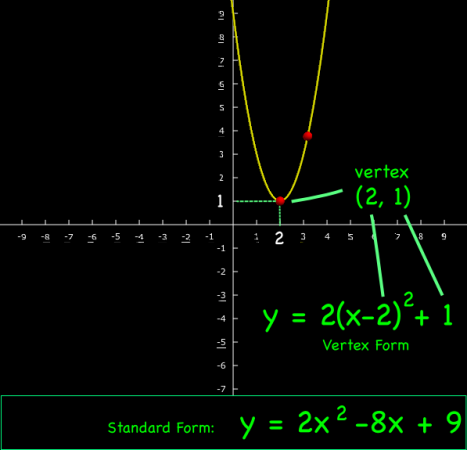
parabola-vertex-eqn — Highlighting the Vertex Form of the equation for a parabola.

The equation for a parabola is usually written as:

Standard form:
$! y = ax^2 + bx + c$

where a, b and c are constants. This is the form displayed in both the VPython Parabola and Excel parabola programs. However, to make the movement of the curve easier, the VPython program also uses the vertex form of the equation internally:

Vertex Form:
$! y = a(x-h)^2 + k$

where the point (h, k) is the location of the vertex of the parabola. In the example above, h = 1 and k = 2.

To translate between the two forms of the equation, you have to rewrite them. Start by expanding the vertex form:

y = a(x – h)² + k

becomes:

y = a(x – h)(x – h) + k

multiplied out to get:

y = a(x² – 2hx + h²) + k

now distribute the a:

y = ax² – 2ahx + ah² + k

finally, group all the coefficients:

y = (a)x² – (2ah)x + (ah² + k)

This equation has the same form as y = ax² + bx + c if:

Vertex to Standard Form:

a = a
b = -2ah
c = ah²+k

And we can rearrange these equations to go the other way, to find the vertex form from the standard form:

Standard to Vertex Form:

$! a = a$
$! h = \frac{\displaystyle -b}{\displaystyle 2a}$
$! k = c - ah^2 = c - \frac{\displaystyle b^2}{\displaystyle 4a}$

Summary

In sum, you can write the standard equation for a parabola as:

Standard form:

And you can write the equation for the same parabola in vertex form as:

Vertex form:

UPDATES

UPDATE 1: This app will automatically convert from standard to vertex form (or back again).

UPDATE 2: Automatically generate and embed graphs using this parabolic grapher app.

Parabola Program

parabola-200b — Animation showing the widening and shrinking of the parabola.

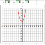
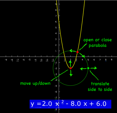
So I put together this interactive parabola program using VPython (code here) for students encountering these curves in Algebra.

It’s a more interactive version of the Excel parabola program in that you can move the curve by dragging on some control points, rather than just having to enter the coefficients of the equation. The program is still in development, but it is at a useful stage right now, so I thought I’d make it available for anyone who wanted to try it.

The program is fairly straightforward to use. You can move the curve (translate it) up and down, and expand or tighten the area within the parabola.

The program also displays the equation of the curve in standard form:
$! y = ax^2 + bx + c$

Next Steps

I’m also working making the standard equation editable by clicking on it and typing, and am considering showing the x-axis intercepts, which will give algebra students a nice, visual way to of checking their factoring.

References

Coffman, J., 2011 (accessed). Translating Parabolas. http://www.jcoffman.com/Algebra2/ch5_3.htm

Math Warehouse, 2011 (accessed). Equation of a Parabola
Standard Form and Vertex Form Equations, http://www.mathwarehouse.com/geometry/parabola/standard-and-vertex-form.php#

WolframAlpha.com, 2011 (accessed). http://www.wolframalpha.com/input/?i=a^2+x^4%2Bx^2-r^2%3D0