Environments for Teaching Python in Middle and High School

I’ve been using python as the primary programming language for all of my classes, from middle to high school. However, with a variety of different machines and operating systems–macs, PC’s, OSX, Windows, ChromeOS–it has been bit of a pain getting everyone up and running and on the same page. It has been especially problematic because I like to use NumPy and, especially, the VPython module because of its nice, easy 3d visualizations.

I’ve tried Anaconda, which works great on some machines but not so much on others. One student with a Mac had to restart the kernel every time he ran a program with vpython, while others had trouble getting it to work properly at all. I do like the way it allows you to put everything into a single Jupyter Notebook, which works nicely for teaching-length programming assignments, but becomes cumbersome for longer projects. Joel Grus goes into detail about why he does not like Notebooks for teaching; much of which I agree with. I do like the Spyder IDE a lot, but I’ve run into some computers that have problems with it (constant crashes).

So, I’ve been using Glowscript a lot with the lower grades. It’s online, so you only need a browser, and its made for vpython, so you can do a lot of the numerical work with it. However, because it’s online you can’t, understandably, get it to write output files to your computer–you have to copy and paste from its output. I’m also not sure how to import user-created modules, which further limits its utility for higher-level classes.

I’ve recently run into repl.it, and I’m having a student try it out in my Numerical Methods class. It looks quite promising as it seems to be able to manage files well and we’ve tried some basic numerical programs using numpy and matplotlib. However, I’ve not got it running vPython yet (although it’s come close).

(repl.it update): One of our other teachers has been trying repl.it with the middle school class and really likes it.

I’ve also recently discovered MakeCode. I’m looking into it for the lower grades, down to 6th grade or even earlier, because it lets you write programs for Minecraft, which is very popular with a remarkably broad age group. It lets you work in blocks, python, or JavaScript. From my poking around, the first couple of things it teaches you to do in Minecraft are write statements (to generate a chicken) and the loops (to generate a lot of chickens). I’ve asked one of my 9th grade, Minecraft players to investigate, so I should have some results to report soon.

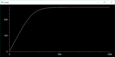
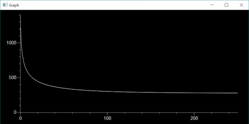
At the moment, for my most advanced class, we’re taking a whatever-works approach. We’re learning about finite differences and using matplotlib to graph the output. I have one student, mentioned above, using repl.it, and another one using Jupyter Notebook on a Mac. A different Mac user is invoking IDLE from the command line because they prefer the IDLE IDE, but couldn’t get numpy to install properly with the python 3.9 version they’d installed earlier–the command-line IDLE actually goes to their Anaconda installation. I have one student, on a Windows machine, for whom everything just works and are using their regular IDLE installation. We spent the entire class period getting everyone up and running with something, but at least now everyone has at least one environment they can use. I’m curious to see what the kids who have multiple options are going to go with.

Modeling Earth’s Energy Balance (Zero-D) (Transient)

Temperature change over time (in thousands of years). As the Earth warms from 3K to equilibrium.

If the Earth behaved as a perfect black body and absorbed all incoming solar radiation (and radiated with 100% emissivity) the we calculated that the average surface temperature would be about 7 degrees Celsius above freezing (279 K). Keeping with this simplification we can think about how the Earth’s temperature could change with time if it was not at equilibrium.

If the Earth started off at the universe’s background temperature of about 3K, how long would it take to get up to the equilibrium temperature?

Using the same equations for incoming solar radiation (Ein) and energy radiated from the Earth (Eout):

 E_{in} = I \times \pi (r_E)^2

 E_{out} = \sigma T^4 4 \pi r_{E}^2

Symbols and constants are defined here except:

  • rE = 6.371 x 10⁶ m

At equilibrium the energy in is equal to the energy out, but if the temperature is 3K instead of 279K the outgoing radiation is going to be a lot less than at equilibrium. This means that there will be more incoming energy than outgoing energy and that energy imbalance will raise the temperature of the Earth. The energy imbalance (ΔE) would be:

 \Delta E = E_{in}-E_{out}

All these energies are in Watts, which as we’ll recall are equivalent to Joules/second. In order to change the temperature of the Earth, we’ll need to know the specific heat capacity (cE) of the planet (how much heat is required to raise the temperature by one Kelvin per unit mass) and the mass of the planet. We’ll approximate the entire planet’s heat capacity with that of one of the most common rocks, granite. The mass of the Earth (mE) we can get from NASA:

  • cE = 800 J/kg/K
  • mE = 5.9723×1024kg

So looking at the units we can figure out the the change in temperature (ΔT) is:

 \Delta T = \frac{\Delta E \Delta t}{c_E m_E}

Where Δt is the time step we’re considering.

Now we can write a little program to model the change in temperature over time:

EnergyBalance.py

from visual import *
from visual.graph import *

I = 1367.
r_E = 6.371E6
c_E = 800.
m_E = 5.9723E24

sigma = 5.67E-8

T = 3                               # initial temperature

yr = 60*60*24*365.25
dt = yr * 100
end_time = yr * 1000000
nsteps = int(end_time/dt)

Tgraph = gcurve()

for i in range(nsteps):
    t = i*dt
    E_in = I * pi * r_E**2
    E_out = sigma * (T**4) * 4 * pi * r_E**2
    dE = E_in - E_out
    dT = dE * dt / (c_E * m_E)
    T += dT
    Tgraph.plot(pos=(t/yr/1000,T))
    if i%10 == 0:
        print t/yr, T
        rate(60)
    

The results of this simulation are shown at the top of this post.

What if we changed the initial temperature from really cold to really hot? When the Earth formed from the accretionary disk of the solar nebula the surface was initially molten. Let’s assume the temperature was that of molten granite (about 1500K).

Cooling if the Earth started off molten (1500K). Note that this simulation only runs for 250,000 years, while the warming simulation (top of page) runs for 1,000,000 years.

Modeling Earth’s Energy Balance (Zero-D) (Equilibrium)

For conservation of energy, the short-wave solar energy absorbed by the Earth equals the long-wave outgoing radiation.

Energy and matter can’t just disappear. Energy can change from one form to another. As a thrown ball moves upwards, its kinetic energy of motion is converted to potential energy due to gravity. So we can better understand systems by studying how energy (and matter) are conserved.

Energy Balance for the Earth

Let’s start by considering the Earth as a simple system, a sphere that takes energy in from the Sun and radiates energy off into space.

Incoming Energy

At the Earth’s distance from the Sun, the incoming radiation, called insolation, is 1367 W/m2. The total energy (wattage) that hits the Earth (Ein) is the insolation (I) times the area the solar radiation hits, which is the area a cross section of the Earth (Acx).

 E_{in} = I \times A_{cx}

Given the Earth’s radius (rE) and the area of a circle, this becomes:

 E_{in} = I \times \pi (r_E)^2

Outgoing Energy

The energy radiated from the Earth is can be calculated if we assume that the Earth is a perfect black body–a perfect absorber and radiatior of Energy (we’ve already been making this assumption with the incoming energy calculation). In this case the energy radiated from the planet (Eout) is proportional to the fourth power of the temperature (T) and the surface area that is radiated, which in this case is the total surface area of the Earth (Asurface):

 E_{out} = \sigma T^4 A_{surface}

The proportionality constant (σ) is: σ = 5.67 x 10⁻⁸ W m-2 K-4

Note that since σ has units of Kelvin then your temperature needs to be in Kelvin as well.

Putting in the area of a sphere we get:

 E_{out} = \sigma T^4 4 \pi r_{E}^2

Balancing Energy

Now, if the energy in balances with the energy out we are at equilibrium. So we put the equations together:

 E_{in} = E_{out}

 I \times \pi r_{E}^2  = \sigma T^4 4 \pi r_{E}^2

cancelling terms on both sides of the equation gives:

 I = 4 \sigma T^4

and solving for the temperature produces:

 T = \sqrt{\frac{I}{4 \sigma}}

Plugging in the numbers gives an equilibrium temperature for the Earth as:

T = 278.6 K

Since the freezing point of water is 273K, this temperature is a bit cold (and we haven’t even considered the fact that the Earth reflects about 30% of the incoming solar radiation back into space). But that’s the topic of another post.

Projectile Paths

Paths of a projectile. The half oval represents a line connecting the maximum heights of each projectile.
Paths of a projectile.

I had my Numerical Methods student calculate the angle that would give a ballistic projectile its maximum range, then I had them write a program that did the the same by just trying a bunch of different angles. The diagram above is what they came up with.

It made an interesting pattern that I converted into a face-plate cover for a light switch that I made using the laser at the TechShop.

Face plate cover.
Face plate cover.

Maximum Range of a Potato Gun

One of the middle schoolers built a potato gun for his math class. He was looking a the mathematical relationship between the amount of fuel (hair spray) and the hang-time of the potato. To augment this work, I had my Numerical Methods class do the math and create analytical and numerical models of the projectile motion.

One of the things my students had to figure out was what angle would give the maximum range of the projectile? You can figure this out analytically by finding the function for how the horizontal distance (x) changes as the angle (theta) changes (i.e. x(theta)) and then finding the maximum of the function.

Initial velocity vector (v) and its component vectors in the x and y directions.
Initial velocity vector (v) and its component vectors in the x and y directions for a given angle.

Distance as a function of the angle

In a nutshell, to find the distance traveled by the potato we break its initial velocity into its x and y components (vx and vy), use the y component to find the flight time of the projectile (tf), and then use the vx component to find the distance traveled over the flight time.

Starting with the diagram above we can separate the initial velocity of the potato into its two components using basic trigonometry:

 \cos{\theta} = \frac{v_x}{v}
 \sin{\theta} = \frac{v_y}{v} ,

so,

 v_x = v \cos{\theta} ,
 v_y = v \sin{\theta}

Now we know that the height of a projectile (y) is given by the function:

! y(t) = \frac{a t^2}{2} + v_0 t + y_0

(you can figure this out by assuming that the acceleration due to gravity (a) is constant and acceleration is the second differential of position with respect to time.)

To find the flight time we assume we’re starting with an initial height of zero (y0 = 0), and that the flight ends when the potato hits the ground which is also at zero ((yt = 0), so:

! 0 = \frac{a t^2}{2} + v_0 t + 0

! 0 = \frac{a t^2}{2} + v_0 t

Factoring out t gives:

! 0 = t ( \frac{a t}{2} + v_0)

Looking at the two factors, we can now see that there are two solutions to this problem, which should not be too much of a surprise since the height equation is parabolic (a second order polynomial). The solutions are when:

! t = 0

!  \frac{a t}{2} + v_0 = 0

The first solution is obviously the initial launch time, while the second is going to be the flight time (tf).

!  \frac{a t_f}{2} + v_0 = 0

!  t_f = - \frac{2 v_0}{a}

You might think it’s odd to have a negative in the equation, but remember, the acceleration is negative so it’ll cancel out.

Now since we’re working with the y component of the velocity vector, the initial velocity in this equation (v0) is really just vy:

!   v_0 = v_y

so we can substitute in the trig function for vy to get:

!  t_f = - \frac{2 v  \sin{\theta}}{a}

Our horizontal distance is simply given by the velocity in the x direction (vx) times the flight time:

!  x = v_x t_f

which becomes:

!  x = v_x  \left(- \frac{2 v  \sin{\theta}}{a}\right)

and substituting in the trig function for vx (just to make things look more complicated):

!  x = \left(  v \cos{\theta} \right)  \left(- \frac{2 v  \sin{\theta}}{a}\right)

and factoring out some of the constants gives:

!  x = -\frac{v^2}{a} 2 \sin{\theta}\cos{theta}

Now we have distance as a function of the launch angle.

We can simplify this a little by using the double-angle formula:

!  \sin{2\theta} = 2 \sin{\theta}\cos{theta}

to get:

!  x = -\frac{v^2}{a} \sin{2\theta}

Finding the maximum distance

How do we find the maxima for this function. Sketching the curve should be easy enough, but because we know a little calculus we know that the maximum will occur when the first differential is equal to zero. So we differentiate with respect to the angle to get:

!  \frac{dx}{d\theta} = -\frac{v^2}{a} 2 \cos{2\theta}

and set the differential equal to zero:

!  0 = -\frac{v^2}{a} 2 \cos{2\theta}

and solve to get:

!  \cos{2\theta}  = 0

!  2\theta  = \cos^{-1}{(0)}

Since we remember that the arccosine of 0 is 90 degrees:

!  2\theta  = 90^{\circ}

!  \theta  = 45^{\circ}

And thus we’ve found the angle that gives the maximum launch distance for a potato gun.

Numerical and Analytical Solutions 2: Constant Acceleration

Previously, I showed how to solve a simple problem of motion at a constant velocity analytically and numerically. Because of the nature of the problem both solutions gave the same result. Now we’ll try a constant acceleration problem which should highlight some of the key differences between the two approaches, particularly the tradeoffs you must make when using numerical approaches.

The Problem

  • A ball starts at the origin and moves horizontally with an acceleration of 0.2 m/s2. Print out a table of the ball’s position (in x) with time (every second) for the first 20 seconds.

Analytical Solution
We know that acceleration (a) is the change in velocity with time (t):

 a = \frac{dv}{dt}

so if we integrate acceleration we can find the velocity. Then, as we saw before, velocity (v) is the change in position with time:

 v = \frac{dx}{dt}

which can be integrated to find the position (x) as a function of time.

So, to summarize, to find position as a function of time given only an acceleration, we need to integrate twice: first to get velocity then to get x.

For this problem where the acceleration is a constant 0.2 m/s2 we start with acceleration:

 \frac{dv}{dt} = 0.2

which integrates to give the general solution,

 v = 0.2 t + c

To find the constant of integration we refer to the original question which does not say anything about velocity, so we assume that the initial velocity was 0: i.e.:

at t = 0 we have v = 0;

which we can substitute into the velocity equation to find that, for this problem, c is zero:

 v = 0.2 t + c
 0 = 0.2 (0) + c
 0 = c

making the specific velocity equation:
 v = 0.2 t

we replace v with dx/dt and integrate:

 \frac{dx}{dt} = 0.2 t
 x = \frac{0.2 t^2}{2} + c
 x = 0.1 t^2 + c

This constant of integration can be found since we know that the ball starts at the origin so

at t = 0 we have x = 0, so;

 x = 0.1 t^2 + c
 0 = 0.1 (0)^2 + c
 0 = c

Therefore our final equation for x is:

 x = 0.1 t^2

Summarizing the Analytical

To summarize the analytical solution:

 a = 0.2
 v = 0.2 t
 x = 0.1 t^2

These are all a function of time so it might be more proper to write them as:

 a(t) = 0.2
 v(t) = 0.2 t
 x(t) = 0.1 t^2

Velocity and acceleration represent rates of change which so we could also write these equations as:

 a(t) = \frac{dv}{dt} = 0.2
 v(t) = \frac{dx}{dt} = 0.2 t
 x(t) = x = 0.1 t^2

or we could even write acceleration as the second differential of the position:

 a(t) = \frac{d^2x}{dt^2} = 0.2
 v(t) = \frac{dx}{dt} = 0.2 t
 x(t) = x = 0.1 t^2

or, if we preferred, we could even write it in prime notation for the differentials:

 a(t) = x''(t) = 0.2
 v(t) = x'(t) = 0.2 t
 x(t) = x(t) =0.1 t^2

The Numerical Solution

As we saw before we can determine the position of a moving object if we know its old position (xold) and how much that position has changed (dx).

 x_{new} = x_{old} + dx

where the change in position is determined from the fact that velocity (v) is the change in position with time (dx/dt):

 v = \frac{dx}{dt}

which rearranges to:

 dx = v dt

So to find the new position of an object across a timestep we need two equations:

 dx = v dt
 x_{new} = x_{old} + dx

In this problem we don’t yet have the velocity because it changes with time, but we could use the exact same logic to find velocity since acceleration (a) is the change in velocity with time (dv/dt):

 a = \frac{dv}{dt}

which rearranges to:

 dv = a dt

and knowing the change in velocity (dv) we can find the velocity using:

 v_{new} = v_{old} + dv

Therefore, we have four equations to find the position of an accelerating object (note that in the third equation I’ve replaced v with vnew which is calculated in the second equation):

 dv = a dt
 v_{new} = v_{old} + dv
 dx = v_{new} dt
 x_{new} = x_{old} + dx

These we can plug into a python program just so:

motion-01-both.py

from visual import *

# Initialize
x = 0.0
v = 0.0
a = 0.2
dt = 1.0

# Time loop
for t in arange(dt, 20+dt, dt):

     # Analytical solution
     x_a = 0.1 * t**2

     # Numerical solution
     dv = a * dt
     v = v + dv
     dx = v * dt
     x = x + dx

     # Output
     print t, x_a, x

which give output of:

>>> 
1.0 0.1 0.2
2.0 0.4 0.6
3.0 0.9 1.2
4.0 1.6 2.0
5.0 2.5 3.0
6.0 3.6 4.2
7.0 4.9 5.6
8.0 6.4 7.2
9.0 8.1 9.0
10.0 10.0 11.0
11.0 12.1 13.2
12.0 14.4 15.6
13.0 16.9 18.2
14.0 19.6 21.0
15.0 22.5 24.0
16.0 25.6 27.2
17.0 28.9 30.6
18.0 32.4 34.2
19.0 36.1 38.0
20.0 40.0 42.0

Here, unlike the case with constant velocity, the two methods give slightly different results. The analytical solution is the correct one, so we’ll use it for reference. The numerical solution is off because it does not fully account for the continuous nature of the acceleration: we update the velocity ever timestep (every 1 second), so the velocity changes in chunks.

To get a better result we can reduce the timestep. Using dt = 0.1 gives final results of:

18.8 35.344 35.532
18.9 35.721 35.91
19.0 36.1 36.29
19.1 36.481 36.672
19.2 36.864 37.056
19.3 37.249 37.442
19.4 37.636 37.83
19.5 38.025 38.22
19.6 38.416 38.612
19.7 38.809 39.006
19.8 39.204 39.402
19.9 39.601 39.8
20.0 40.0 40.2

which is much closer, but requires a bit more runtime on the computer. And this is the key tradeoff with numerical solutions: greater accuracy requires smaller timesteps which results in longer runtimes on the computer.

Post Script

To generate a graph of the data use the code:

from visual import *
from visual.graph import *

# Initialize
x = 0.0
v = 0.0
a = 0.2
dt = 1.0

analyticCurve = gcurve(color=color.red)
numericCurve = gcurve(color=color.yellow)
# Time loop
for t in arange(dt, 20+dt, dt):

     # Analytical solution
     x_a = 0.1 * t**2

     # Numerical solution
     dv = a * dt
     v = v + dv
     dx = v * dt
     x = x + dx

     # Output
     print t, x_a, x
     analyticCurve.plot(pos=(t, x_a))
     numericCurve.plot(pos=(t,x))

which gives:

Comparison of numerical and analytical solutions using a timestep (dt) of 1.0 seconds.

Numerical versus Analytical Solutions

We’ve started working on the physics of motion in my programming class, and really it boils down to solving differential equations using numerical methods. Since the class has a calculus co-requisite I thought a good way to approach teaching this would be to first have the solve the basic equations for motion (velocity and acceleration) analytically–using calculus–before we took the numerical approach.

Constant velocity

  • Question 1. A ball starts at the origin and moves horizontally at a speed of 0.5 m/s. Print out a table of the ball’s position (in x) with time (t) (every second) for the first 20 seconds.

Analytical Solution:
Well, we know that speed is the change in position (in the x direction in this case) with time, so a constant velocity of 0.5 m/s can be written as the differential equation:

 \frac{dx}{dt} = 0.5

To get the ball’s position at a given time we need to integrate this differential equation. It turns out that my calculus students had not gotten to integration yet. So I gave them the 5 minute version, which they were able to pick up pretty quickly since integration’s just the reverse of differentiation, and we were able to move on.

Integrating gives:

 x = 0.5t + c

which includes a constant of integration (c). This is the general solution to the differential equation. It’s called the general solution because we still can’t use it since we don’t know what c is. We need to find the specific solution for this particular problem.

In order to find c we need to know the actual position of the ball is at one point in time. Fortunately, the problem states that the ball starts at the origin where x=0 so we know that:

  • at t = 0, x = 0

So we plug these values into the general solution to get:

 0 = 0.5(0) + c
solving for c gives:

 c = 0

Therefore our specific solution is simply:

 x = 0.5t

And we can write a simple python program to print out the position of the ball every second for 20 seconds:

motion-01-analytic.py

for t in range(21):
     x = 0.5 * t
     print t, x

which gives the result:

>>> 
0 0.0
1 0.5
2 1.0
3 1.5
4 2.0
5 2.5
6 3.0
7 3.5
8 4.0
9 4.5
10 5.0
11 5.5
12 6.0
13 6.5
14 7.0
15 7.5
16 8.0
17 8.5
18 9.0
19 9.5
20 10.0

Numerical Solution:
Finding the numerical solution to the differential equation involves not integrating, which is particularly good if the differential equation can’t be integrated.

We start with the same differential equation for velocity:
 \frac{dx}{dt} = 0.5

but instead of trying to solve it we’ll just approximate a solution by recognizing that we use dx/dy to represent when the change in x and t are really, really small. If we were to assume they weren’t infinitesimally small we would rewrite the equations using deltas instead of d’s:
 \frac{\Delta x}{\Delta t} = 0.5

now we can manipulate this equation using algebra to show that:
 \Delta x = 0.5 \Delta t

so the change in the position at any given moment is just the velocity (0.5 m/s) times the timestep. Therefore, to keep track of the position of the ball we need to just add the change in position to the old position of the ball:

 x_{new} = x_{old} + \Delta x

Now we can write a program to calculate the position of the ball using this numerical approximation.

motion-01-numeric.py

from visual import *

# Initialize
x = 0.0
dt = 1.0

# Time loop
for t in arange(dt, 21, dt):
     v = 0.5
     dx = v * dt
     x = x + dx
     print t, x

I’m sure you’ve noticed a couple inefficiencies in this program. Primarily, that the velocity v, which is a constant, is set inside the loop, which just means it’s reset to the same value every time the loop loops. However, I’m putting it in there because when we get working on acceleration the velocity will change with time.

I also import the visual library (vpython.org) because it imports the numpy library and we’ll be creating and moving 3d balls in a little bit as well.

Finally, the two statements for calculating dx and x could easily be combined into one. I’m only keeping them separate to be consistent with the math described above.

A Program with both Analytical and Numerical Solutions
For constant velocity problems the numerical approach gives the same results as the analytical solution, but that’s most definitely not going to be the case in the future, so to compare the two results more easily we can combine the two programs into one:

motion-01.py

from visual import *
# Initialize
x = 0.0
dt = 1.0

# Time loop
for t in arange(dt, 21, dt):
     v = 0.5

     # Analytical solution
     x_a = v * t

     # Numerical solution
     dx = v * dt
     x = x + dx

     # Output
     print t, x_a, x

which outputs:

>>> 
1.0 0.5 0.5
2.0 1.0 1.0
3.0 1.5 1.5
4.0 2.0 2.0
5.0 2.5 2.5
6.0 3.0 3.0
7.0 3.5 3.5
8.0 4.0 4.0
9.0 4.5 4.5
10.0 5.0 5.0
11.0 5.5 5.5
12.0 6.0 6.0
13.0 6.5 6.5
14.0 7.0 7.0
15.0 7.5 7.5
16.0 8.0 8.0
17.0 8.5 8.5
18.0 9.0 9.0
19.0 9.5 9.5
20.0 10.0 10.0

Solving a problem involving acceleration comes next.

Experimenting with Genetic Algorithms

Genetic algorithm trying to find a series of four mathematical operations (e.g. -3*4/7+9) that would result in the number 42.

I’m teaching a numerical methods class that’s partly an introduction to programming, and partly a survey of numerical solutions to different types of problems students might encounter in the wild. I thought I’d look into doing a session on genetic algorithms, which are an important precursor to things like networks that have been found to be useful in a wide variety of fields including image and character recognition, stock market prediction and medical diagnostics.

The ai-junkie, bare-essentials page on genetic algorithms seemed a reasonable place to start. The site is definitely readable and I was able to put together a code to try to solve its example problem: to figure out what series of four mathematical operations using only single digits (e.g. +5*3/2-7) would give target number (42 in this example).

The procedure is as follows:

  • Initialize: Generate several random sets of four operations,
  • Test for fitness: Check which ones come closest to the target number,
  • Select: Select the two best options (which is not quite what the ai-junkie says to do, but it worked better for me),
  • Mate: Combine the two best options semi-randomly (i.e. exchange some percentage of the operations) to produce a new set of operations
  • Mutate: swap out some small percentage of the operations randomly,
  • Repeat: Go back to the second step (and repeat until you hit the target).

And this is the code I came up with:

genetic_algorithm2.py

''' Write a program to combine the sequence of numbers 0123456789 and
    the operators */+- to get the target value (42 (as an integer))
'''

'''
Procedure:
    1. Randomly generate a few sequences (ns=10) where each sequence is 8
       charaters long (ng=8).
    2. Check how close the sequence's value is to the target value.
        The closer the sequence the higher the weight it will get so use:
            w = 1/(value - target)
    3. Chose two of the sequences in a way that gives preference to higher
       weights.
    4. Randomly combine the successful sequences to create new sequences (ns=10)
    5. Repeat until target is achieved.

'''
from visual import *
from visual.graph import *
from random import *
import operator

# MODEL PARAMETERS
ns = 100
target_val = 42 #the value the program is trying to achieve
sequence_length = 4  # the number of operators in the sequence
crossover_rate = 0.3
mutation_rate = 0.1
max_itterations = 400


class operation:
    def __init__(self, operator = None, number = None, nmin = 0, nmax = 9, type="int"):
        if operator == None:
            n = randrange(1,5)
            if n == 1:
                self.operator = "+"
            elif n == 2:
                self.operator = "-"
            elif n == 3:
                self.operator = "/"
            else:
                self.operator = "*"
        else:
            self.operator = operator
            
        if number == None:
            #generate random number from 0-9
            self.number = 0
            if self.operator == "/":
                while self.number == 0:
                    self.number = randrange(nmin, nmax)
            else:
                self.number = randrange(nmin, nmax)
        else:
            self.number = number
        self.number = float(self.number)

    def calc(self, val=0):
        # perform operation given the input value
        if self.operator == "+":
            val += self.number
        elif self.operator == "-":
            val -= self.number
        elif self.operator == "*":
            val *= self.number
        elif self.operator == "/":
            val /= self.number
        return val


class gene:

    def __init__(self, n_operations = 5, seq = None):
        #seq is a sequence of operations (see class above)
        #initalize
        self.n_operations = n_operations
        
        #generate sequence
        if seq == None:
            #print "Generating sequence"
            self.seq = []
            self.seq.append(operation(operator="+"))  # the default operation is + some number
            for i in range(n_operations-1):
                #generate random number
                self.seq.append(operation())

        else:
            self.seq = seq

        self.calc_seq()

        #print "Sequence: ", self.seq
    def stringify(self):
        seq = ""
        for i in self.seq:
            seq = seq + i.operator + str(i.number)
        return seq

    def calc_seq(self):
        self.val = 0
        for i in self.seq:
            #print i.calc(self.val)
            self.val = i.calc(self.val)
        return self.val

    def crossover(self, ingene, rate):
        # combine this gene with the ingene at the given rate (between 0 and 1)
        #  of mixing to create two new genes

        #print "In 1: ", self.stringify()
        #print "In 2: ", ingene.stringify()
        new_seq_a = []
        new_seq_b = []
        for i in range(len(self.seq)):
            if (random() < rate): # swap
                new_seq_a.append(ingene.seq[i])
                new_seq_b.append(self.seq[i])
            else:
                new_seq_b.append(ingene.seq[i])
                new_seq_a.append(self.seq[i])

        new_gene_a = gene(seq = new_seq_a)
        new_gene_b = gene(seq = new_seq_b)
                       
        #print "Out 1:", new_gene_a.stringify()
        #print "Out 2:", new_gene_b.stringify()

        return (new_gene_a, new_gene_b)

    def mutate(self, mutation_rate):
        for i in range(1, len(self.seq)):
            if random() < mutation_rate:
                self.seq[i] = operation()


def weight(target, val):
    if val <> None:
        #print abs(target - val)
        if abs(target - val) <> 0:
            w = (1. / abs(target - val))
        else:
            w = "Bingo"
            print "Bingo: target, val = ", target, val
    else:
        w = 0.
    return w

def pick_value(weights):
    #given a series of weights randomly pick one of the sequence accounting for
    # the values of the weights

    # sum all the weights (for normalization)
    total = 0
    for i in weights:
        total += i

    # make an array of the normalized cumulative totals of the weights.
    cum_wts = []
    ctot = 0.0
    cum_wts.append(ctot)
    for i in range(len(weights)):
        ctot += weights[i]/total
        cum_wts.append(ctot)
    #print cum_wts

    # get random number and find where it occurs in array
    n = random()
    index = randrange(0, len(weights)-1)
    for i in range(len(cum_wts)-1):
        #print i, cum_wts[i], n, cum_wts[i+1]
        if n >= cum_wts[i] and n < cum_wts[i+1]:
            
            index = i
            #print "Picked", i
            break
    return index

def pick_best(weights):
    # pick the top two values from the sequences
    i1 = -1
    i2 = -1
    max1 = 0.
    max2 = 0.
    for i in range(len(weights)):
        if weights[i] > max1:
            max2 = max1
            max1 = weights[i]
            i2 = i1
            i1 = i
        elif weights[i] > max2:
            max2 = weights[i]
            i2 = i

    return (i1, i2)


# Main loop
l_loop = True
loop_num = 0
best_gene = None

##test = gene()
##test.print_seq()
##print test.calc_seq()

# initialize
genes = []
for i in range(ns):
    genes.append(gene(n_operations=sequence_length))
    #print genes[-1].stringify(), genes[-1].val
    

f1 = gcurve(color=color.cyan)

while (l_loop and loop_num < max_itterations):
    loop_num += 1
    if (loop_num%10 == 0):
        print "Loop: ", loop_num

    # Calculate weights
    weights = []
    for i in range(ns):
        weights.append(weight(target_val, genes[i].val))
        # check for hit on target
        if weights[-1] == "Bingo":
            print "Bingo", genes[i].stringify(), genes[i].val
            l_loop = False
            best_gene = genes[i]
            break
    #print weights

    if l_loop:

        # indicate which was the best fit option (highest weight)
        max_w = 0.0
        max_i = -1
        for i in range(len(weights)):
            #print max_w, weights[i]
            if weights[i] > max_w:
                max_w = weights[i]
                max_i = i
        best_gene = genes[max_i]
##        print "Best operation:", max_i, genes[max_i].stringify(), \
##              genes[max_i].val, max_w
        f1.plot(pos=(loop_num, best_gene.val))


        # Pick parent gene sequences for next generation
        # pick first of the genes using weigths for preference    
##        index = pick_value(weights)
##        print "Picked operation:  ", index, genes[index].stringify(), \
##              genes[index].val, weights[index]
##
##        # pick second gene
##        index2 = index
##        while index2 == index:
##            index2 = pick_value(weights)
##        print "Picked operation 2:", index2, genes[index2].stringify(), \
##              genes[index2].val, weights[index2]
##

        (index, index2) = pick_best(weights)
        
        # Crossover: combine genes to get the new population
        new_genes = []
        for i in range(ns/2):
            (a,b) = genes[index].crossover(genes[index2], crossover_rate)
            new_genes.append(a)
            new_genes.append(b)

        # Mutate
        for i in new_genes:
            i.mutate(mutation_rate)
                

        # update genes array
        genes = []
        for i in new_genes:
            genes.append(i)


print
print "Best Gene:", best_gene.stringify(), best_gene.val
print "Number of iterations:", loop_num
##

When run, the code usually gets a valid answer, but does not always converge: The figure at the top of this post shows it finding a solution after 142 iterations (the solution it found was: +8.0 +8.0 *3.0 -6.0). The code is rough, but is all I have time for at the moment. However, it should be a reasonable starting point if I should decide to discuss these in class.