Dilation

Dilation (scaling) of a quadrilateral by 2x.

A quick program that animates scaling (dilation) of shapes by scaling the coordinates. You type in the dilation factor.

dilation.py

from visual import *

#axes
xmin = -10.
xmax = 10.
ymin = -10.
ymax = 10.
xaxis = curve(pos=[(xmin,0),(xmax,0)])
yaxis = curve(pos=[(0,ymin),(0,ymax)])

#tick marks
tic_dx = 1.0
tic_h = .5
for i in arange(xmin,xmax+tic_dx,tic_dx):
    tic = curve(pos=[(i,-0.5*tic_h),(i,0.5*tic_h)])
for i in arange(ymin,ymax+tic_dx,tic_dx):
    tic = curve(pos=[(-0.5*tic_h,i),(0.5*tic_h,i)])

#stop scene from zooming out too far when the curve is drawn
scene.autoscale = False

# define curve here
shape = curve(pos=[(-1,2), (5,3), (4,-1), (-1,-1)])

shape.append(pos=shape.pos[0])
shape.color = color.yellow
shape.radius = 0.1
shape.visible = True

#dilated shape
dshape = curve(color=color.green, radius=shape.radius*0.9)
for i in shape.pos:
    dshape.append(pos=i)

#label
note = label(pos=(5,-8),text="Dilation: 1.0", box=False)
intext = label(pos=(5,-9),text="> x", box=False)

#scaling lines
l_scaling = False
slines = []
for i in range(len(shape.pos)):
    slines.append(curve(radius=shape.radius*.5,color=color.red, pos=[shape.pos[i],shape.pos[i],shape.pos[i]]))


#animation parameters
animation_time = 1. #seconds
animation_smootheness = 30
animation_rate = animation_smootheness / animation_time

x = ""
while 1:
    #x = raw_input("Enter Dilation: ")
    if scene.kb.keys: # event waiting to be processed?
        s = scene.kb.getkey() # get keyboard info

        #print s
        if s <> '\n':
            x += s
            intext.text = "> x "+x
        else:
            try:
                xfloat = float(x)
                note.text = "Dilation: " + x

                endpoints = []
                dp = []
                for i in shape.pos:
                    endpoints.append(float(x) * i)
                    dp.append((endpoints[-1]-i)/animation_smootheness)
                #print "endpoints: ", endpoints
                #print "dp:        ", dp
                for i in range(animation_smootheness):
                    for j in range(len(dshape.pos)):
                        dshape.pos[j] = i*dp[j]+shape.pos[j]
                    rate(animation_smootheness)
                    if slines:
                        for i in range(len(shape.pos)):
                            slines[i].pos[1] = vector(0,0)
                            slines[i].pos[-1] = dshape.pos[i]

                for i in range(len(shape.pos)):
                    dshape.pos[i] = endpoints[i]
                    slines[i].pos[-1] = dshape.pos[i]

                for i in range(len(shape.pos)-1):
                    print shape.pos[i], "--->", dshape.pos[i]
                    
            except:
                #print "FAIL"
                failed = True
                intext.text = "> x "
            x = ""


Transformations and 3D Printing

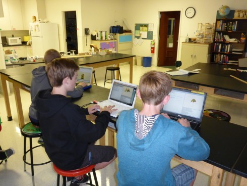
My pre-algebra class is working on transformations, so it seemed a good opportunity to try some 3d printing. I showed them how to create basic shapes (sphere, triangle, and box) and how to move them (transform) in a three-dimensional coordinate system using OpenScad.

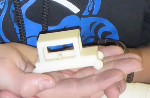
Students create their car models using OpenScad.

Then we started printing them out on our 3d printer. Since it takes about an hour to print each model, we’re printing one or two per day.

The students were quite enthused. The initial OpenScad lesson took about 15 minutes, and I gave them another 55 minutes of class-time to work on them with my help. Now they’re on their own, more or less: they’ll be able to make time if they get their other math work done. A couple of them also came back into the classroom at the end of school today to work on their models.

Our first 3d printed car model.

And I think they learned a bit about transformations in space.

Toothpick Shapes’ Sequences

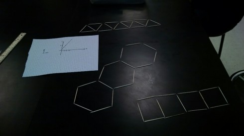
Toothpick shape sequences.

Using a sequence of connected shapes to introduce algebra and graphing to pre-Algebra students.

Make a geometric shape–a square perhaps–out of toothpicks. Count the sides–4 for a square. Now add another square, attached to the first. You should now have 7 toothpicks. Keep adding shapes in a line and counting toothpicks. Now you can:

  • make a table of shapes versus toothpicks,
  • write the sequence as an algebraic expression
  • graph the number of shapes versus the number of toothpicks (it should be a straight line),
  • figure out that the increment of the sequence–3 for a square–is the slope of the line.
  • show that the intercept of the line is when there are zero shapes.

Then I had my students set up a spreadsheet where they could enter the number of shapes and it would give the number of toothpicks needed. Writing a small program to do the same works is the next step.

Practicing Plotting Points on the Co-ordinate Plain

Pre-Algebra class starts next week, so in preparation for one of the early lessons on how to plot x,y co-ordinates, I put together an interactive plotter that lets students drag points onto the co-ordinate plain.

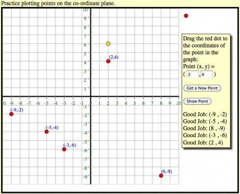
Students practice plotting points by dragging the red dot to the coordinates given.

Usage

The program generates random coordinate pairs within the area of the chart (or you can enter values of the coordinates yourself):

  • Clicking the “Show Point” button will place a yellow dot at the point.
  • When you’re confident you understand how the coordinate pairs work, you can practice by dragging the red dot to where you think the point is and the program will tell you if you’re right or not.

About the Program

This interactive application uses the jQuery and KineticJS javascript libraries. The latter library in particular is useful for making the HTML5 canvases interactive, so you can click on points on the graph and drag them.

When I have some time, after classes settle down, I’ll see if I can figure out how to embed this type of app into this (WordPress) blog. KineticJS is based off HTML5 canvases, which is what I use for the other interactive graphs I’ve posted, so it shouldn’t be terribly hard (at least in principle).

A Review of Fractions: Based on Khan Academy Lessons

This is a basic review of working with fractions using lessons and practice sets from the Khan Academy.

1. Adding Fractions with a Common Denominator

The first topic — adding fractions –ought to be really easy for algebra students, but it allows them to become familiar with the Khan Academy website and doing the practice sets.

Now do the Practice Set.

OPTIONAL: Subtracting fractions with a common denominator works the same way. Students may do this practice set if they find it useful.

2. Adding Fractions with a Different Denominator

This is usually a helpful review.

The practice set.

3. Multiplying and Dividing Fractions

A good review that helps build up to working with radical numbers.

Multiplying fractions:

Do the multiplying fractions practice set.

Dividing Fractions:

Dividing fractions practice set.

4. Converting Fractions to Decimals

The last review is on how to convert fractions to decimals.

Now try the practice set for ordering numbers.

5. Next: Working with Square Roots

Algebra in Programming, and a First Box

One of the first things you learn in algebra is to use variables to represent numbers. Variables are at the heart of computer programming, and in Python you can use them for more than just numbers. So open the IDLE text editor and get to work.

But first we’ll start with numbers. To assign a number to a variable you just write an equation. Here are a couple (you can copy and paste the code into the IDLE window, but usually typing it in yourself tends to be more meaningful and help you remember):

a = 2
b = 3

Now we can add these two variables together and create a new variable c.

a = 2
b = 3
c = a + b

Which is all very nice, but now we want our program to actually tell us what the result is so we print it to the screen.

a = 2
b = 3
c = a + b
print c

Run this program (F5 or select “Run Module” in the “Run” menu) to get:

Output from the first program: 2+3=5.

Basic Operations and Types of Numbers

Now try some other basic operations:

+ and – are easy as you’ve seen above.

× : for multiplication use *, as in:

a = 2
b = 3
c = a * b
print c

÷ : to divide use a /, as in:

a = 2
b = 3
c = a / b
print c

Now as you know, 2 divided by 3 should give you two thirds, but the running this program outputs 0:

2 divided by 3 to gives 0 because Python thinks we're working with integers.

This is because the Python thinks you’re using integers (a whole number), so it gives you an integer result. If you want a fraction in your result, you need to indicate that you’re using real numbers, or more specifically, rational numbers, which can be integers or fractions, but usually show up as a decimal (these are usually referred to as floating point numbers in programming).

The easiest way to indicate that you don’t just want integers is to make one of your original numbers a decimal:

a = 2.0
b = 3
c = a / b
print c

which produces:

Use a = 2.0 to indicate that we're using rational numbers.

Other Things Can Be Variables

In object oriented programming languages like Python you can assign all sorts of things to variables, not just numbers.

To create a box and give it a variable name you can use the program:

from visual import *
c = box()

which produces:

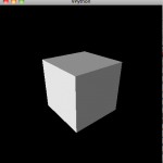
A box created with VPython. It looks much more interesting if you rotate it to see it in perspective.

A rotated, zoomed-out view of a box.

To rotate the view, hold down and drag the right mouse button. To zoom in or out, hold down the right and left buttons together and drag in and out. Mac users will probably have to use the “option” button to zoom, and the “command” button to rotate.

The line from visual import * tells the computer that it needs to use all the stuff in the module called “visual”, which has all the commands to make 3d objects (the “*” indicates all).

The c = box() line creates the box and assigns it a variable name of c. You don’t just have to use letters as variable names. In programming you want to use variable names that will remind you of what it’s supposed to represent. So you could just as well have named your variable “mybox” and gotten the same result:

from visual import *
mybox = box()

Now objects like this box have properties, like color. To make the box red you set the color property in one of two ways. The first method is to set the color as you create the object:

from visual import *
mybox = box(color = color.red)

The second is to set the property using the variable you’ve created and “dot” (.) notation.

from visual import *
mybox = box()
mybox.color = color.red

In both of these color.red is a variable name that the computer already knows because it was imported when you imported the “visual” module. There are a few other named colors like color.green and color.blue that you can find out more about in the VPython documentation (specifically here).

You can also find out about the other properties boxes have, like length, width and position (pos), as well as all the other objects you can create, such as springs, arrows and spheres.

At this point, its probably worth spending a little time creating new objects, and varying their properties.

Overview

We’ve just covered:

  • Assigning values to variables
  • Basic operations (+,-,×, and ÷)
  • Types of Numbers: Integers versus floating point
  • Assigning 3d objects to variables
  • Setting properties of 3d objects

Next we’ll try to make things move.

References

For how to install and run VPython, check here.

Concept Maps of Math

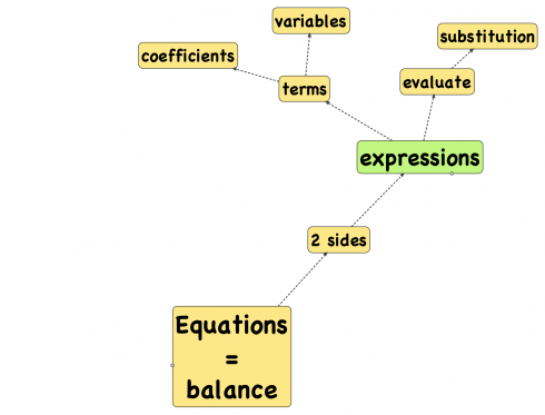
Introduction to algebra.

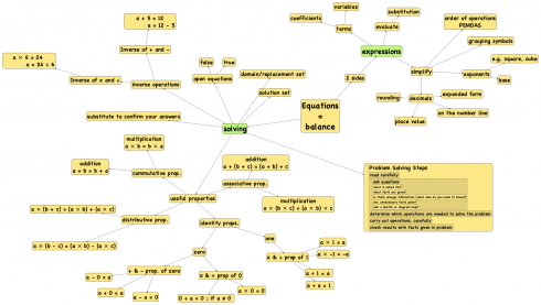
While it’s nice to have the math concepts arranged nicely based on their presentation in the textbook. Since my plan is to give just a few overview lessons and let students discover the details I’ll be presenting things a little differently based on my own conceptual organization. So I’ve created a second graphic map, which looks a bit disorganized, but gives links things by concept, at least in the way I see it.

Concept map for an introduction to pre-Algebra based on the first chapter of the textbook, Pre-Algebra an Accelerated Course, by Dolciani et al., (1996).

This morning I presented just the first branch, about equations, expressions and variables. The general discussion covered enough to give the students a good overview of the introduction to Algebra. Tomorrow the pre-Algebra and Algebra topics will start to diverge, but I think today went pretty well.

We’ll see how it goes as we fill in the rest of the map.