Modeling Data with Straight Lines using Excel

Microsoft Excel, like most graphical calculators and spreadsheet programs, has the built in ability to do linear regression of measured data using certain types of functions — lines, polynomials, logarithms, and exponents for example. However, you can get it to do any type of function — sinusoidal, natural log, whatever — if you work through the spreadsheet and can use the iterative Solver tool.

This more general approach is quite useful in teaching pre-Calculus, because the primary purpose of all the functions they have to learn is to create mathematical models (functions) based on data that can be used for predictions.

The Data

I started this year’s pre-calculus class by having them collect some data. In a simplification of the snow-melt experiment I did with the middle school last year, I had them put a beaker of water (about 300ml) on a hot plate and measure the temperature every minute as warmed up.

To make the experiment a little more interesting, I had each student in each group of four take just three consecutive measurements and try to find the equation of the straight line that best fit their data, and could be used to try to predict the other measurements of their peers in their group.

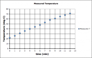
Tvt-scatter — Figure 1. Scatter plot of measured temperatures during the warming of a beaker of water on a hot plate. Data given in Table 1.

It did not quite work out as I’d hoped. Since you only need two points to find the equation of a straight line, having three points produced a little confusion. I’d hoped to produce that confusion, but hadn’t realized that I’d need to do a review of how to find the equation of a straight line. A large fraction of the class was a little bit rusty after hot months of summer.

So, we pooled all the data and reviewed how to find the equation of a straight line.

Table 1: The Data

Time (minutes)	Measured Temperature (°C)
0	22
1	26
2	31
3	36
4	40
5	44
6	48
7	53
8	58
9	61
10	65
11	68
12	71

Finding the Equation for a Straight Line using Two Points

The general equation for a straight lines is:

(1) $y = mx + b$

and we need to determine the coefficients m and b. m is the slope, which can be calculated from two points using the equation:

(2) $m = \frac{y_2 - y_1}{x_2 - x_1}$

using the points at t=6 and t=11 — the points (x₁, y₁) = (6,48) and (x₂, y₂) = (11,68) respectively — for example, gives a slope of:

$m = \frac{68 - 48}{11 - 6}$

$m = \frac{20}{5}$

$m = 4$

so our general equation becomes:

$y = 4 x + b$

to find b we substitute either one of the points into the equation for x and y. If we use the first point, x = 6, and y = 48, we get:

$48 = 4 (6) + b$
$48 = 24 + b$

$24 + b = 48$
$b = 48 - 24$
$b = 24$

and the equation of our line becomes:
(3) $y = 4 x + 24$

Now, since we’re actually looking at a relationship between temperature and time, with temperature on the y-axis and time on the x-axis, we could relabel the terms in the equation with T = temperature and t = time to have:

(4) $T = 4 t + 24$

While this equation is more satisfying to me, because I think it better describes the relationship we have, the more vocal students preferred the equation in terms of x and y (Eqn 3). These are the terms they are more familiar with in the context of a math class, and I recall seeing some evidence that students seem to learn better with the more abstract representations sometimes (though I can’t quite remember the source; I should have blogged about it).

Plotting the Data and the Modeled Straight Line

The straight line equation we came up with (Eqn. 4) is our model of the data. It’s not quite perfect. All the data do not lie on the line, although, if we did everything right, only the points (6, 48) and (11, 68) are guaranteed to be on the line.

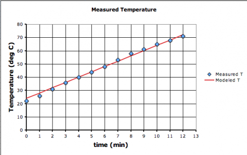
Tvt-mvm — Figure 2. The equation of our straight line model (red line) matches the data (blue diamonds) pretty well.

I showed the class how to plot the scatter graph using MS Excel, and how to draw the line to show the modeled data. The measured data are represented as points since the measurements were made at discrete points in time. The modeled equation, however, is a continuous function, hence the straight line. The Excel sheet below (Resource 1) illustrates:

Resource 1: Excel Spreadsheet of Measured versus Modeled Data

The Best Fit Curve

The Excel spreadsheet (Resource 1) was set up so that when I entered the slope (m) and intercept (b) values, the graph would quickly update. So I went through the class. Everyone called out their slope and intercept values, I plugged them in, and they could all see how the modeled line changed slightly based on the points used to calculate it. So I put the question to them, “How can we figure out which model equation is the best?”

That’s how I was able to introduce the topic of error. What if we compared the temperature predicted by the model for each data point, to the actual value. The smaller the difference in modeled versus measured temperatures, the better the fit of the model. Indeed, if we sum all the differences, or better yet take the average of the differences, we could get a single number, we’ll call the average error (ε), that could be used to compare the different models. I used this opportunity to introduce sigma notation, which the pre-calculus students had not seen much of before.

As a first pass (which, as we’ll see below, has a major problem), the error (ε) for each point (i) is:

$\epsilon_i = (T_{measured}-T_{modeled})$

The average error is the sum of all the errors divided by the number of points (n) (we have 12 points so n=12 in this example):

(5) $\bar{\epsilon} = \frac{\sum\limits_{i=1}^{n} \epsilon_i}{n}$

Now this works, but there is one problem. I was quite pleased and a little bit surprise that one of my students recognized what it was without any coaxing and also suggested a solution: by simply taking the difference to calculate the error, a point that is offset above the modeled line can be canceled out by a point offset by the same amount below the line. So what we really need is to use the absolute value of the error.

(6) $\epsilon_i = \left| T_{measured}-T_{modeled} \right|$

This works, and is what we went with, but I did also point that what’s usually done is to use the square of the error instead of the absolute value. Squaring makes any number positive, so it accomplishes the same goal as the absolute value, and is the approach we’ll use when I go into linear regression later on.

Setting up the Excel spreadsheet to calculate the average error is fairly straightforward as shown in Resource 2:

Resource 2. Calculating the average error using Excel.

So once again, we went through the class and everyone called out their slope and intercept values and cheered when I plugged the numbers in and they saw if they had the lowest value.

It is important to remember, though, that the competition gives a somewhat random result: students’ average error is a function of the points they happened to pick, not how well they did the math (assuming everyone did the math correctly).

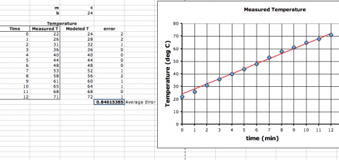
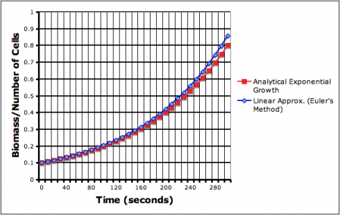
Tvt-sheet — Figure 2. Showing the spreadsheet used to calculate the average error (Resource 2).

Exponential Growth/Decay Models (Summary)

A quick summary (more details here):

The equation that describes exponential growth is:
Exponential Growth: $N = N_0 e^{rt}$

where:

N = number of cells (or concentration of biomass);
N₀ = the starting number of cells;
r = the rate constant, which determines how fast growth occurs; and
t = time.

You can set the r value, but that’s a bit abstract so often these models will use the doubling time – the time it takes for the population (the number of cells, or whatever, to double). The doubling time (t_d) can be calculated from the equation above by:

$t_d = \frac{\ln 2}{r}$

or if you know the doubling time you can find r using:

$r = \frac{\ln 2}{t_d}$

Finally, note that the only difference between a growth model and a decay model is the sign on the exponent:

Exponential Decay: $N = N_0 e^{-rt}$

Decay models have a half-life — the time it takes for half the population to die or change into something else.

Exponential Cell Growth

The video shows 300 seconds of purely exponential growth (uninhibited), captured from the exponential growth VAMP scenario. Like the exponential growth function itself, the video starts off slowly then gets a lot more exciting (for a given value of exciting).

The modeled growth is based on the exponential growth function:

$N = N_0 e^{rt}$ (1)

where:

N = number of cells (or concentration of biomass);
N₀ = the starting number of cells;
r = the rate constant, which determines how fast growth occurs; and
t = time.

Finding the Rate Constant/Doubling Time (r)

You can enter either the rate constant (r) or the doubling time of the particular organism into the model. Determining the doubling time from the exponential growth equation is a nice exercise for pre-calculus students.

Let’s call the doubling time, t_d. When the organism doubles from it’s initial concentration the growth equation becomes:

$2N_0 = N_0 e^{r t_d}$

divide through by N₀:

$2 = e^{r t_d}$

take the natural logs of both sides:

$\ln 2 = \ln (e^{r t_d})$

bring the exponent down (that’s one of the rules of logarithms);

$\ln 2 = r t_d \ln (e)$

remember that ln(e) = 1:

$\ln 2 = r t_d$

and solve for the doubling time:

$\frac{\ln 2}{r} = t_d$

Decay

A nice follow up would be to solve for the half life given the exponential decay function, which differs from the exponential growth function only by the negative in the exponent:

$N = N_0 e^{-rt}$

The UCSD math website has more details about Exponential Growth and Decay.

Finding the Growth Rate

A useful calculus assignment would be to determine the growth rate at any point in time, because that’s what the model actually uses to calculate the growth in cells from timestep to timestep.

The growth rate would be the change in the number of cells with time:

$\frac{dN}{dt}$

starting with the exponential growth equation:

$N = N_0 e^{rt}$

since we have a natural exponent term, we’ll use the rule for differentiating natural exponents:

$\frac{d}{dx}(e^u) = e^u \frac{du}{dx}$

So to make this work we’ll have to define:

$u = rt$

which can be differentiated to give:

$\frac{du}{dt} = r$

and since N₀ is a constant:

$N = N_0 e^{u}$

$\frac{dN}{dt} = N_0 e^{u} \frac{du}{dt}$

substituting in for u and du/dt gives:

$\frac{dN}{dt} = N_0 e^{rt} (r)$

rearranging (to make it look prettier (and clearer)):

$\frac{dN}{dt} = N_0 r e^{rt}$ (2)

Numerical Methods: Euler’s method

With this formula, the model could use linear approximations — like in Euler’s method — to simulate the growth of the biomass.

First we can discretize the differential so that the change in N and the change in time (t$) take on discrete values:
$\frac{dN}{dt} = \frac{\Delta N}{\Delta t}$

Now the change in N is the difference between the current value N^t and the new value N^t+1:

Now using this in our differentiated equation (Eq. 2) gives:

$\frac{N^{t+1}-N^t}{\Delta t} = N_0 r e^{r\Delta t}$

Which we can solve for the new biomass (N^^t+1):

$N^{t+1}-N^t = N_0 r e^{r\Delta t} \Delta t$

to get:
$N^{t+1} = N_0 r e^{r\Delta t} \Delta t + N^t$

This linear approximation, however, does introduce some error.

The approximated exponential growth curve (blue line) deviates from the analytical equation. The deviation compounds itself, getting worse exponentially, as time goes on.

Excel file for graphed data: exponential_growth.xls

VAMP

This is the first, basic but useful product of my summer work on the IMPS website, which is centered on the VAMP biochemical model. The VAMP model is, as of this moment, still in it’s alpha stage of development — it’s not terribly user-friendly and is fairly limited in scope — but is improving rapidly.

The Mathematical Logic Behind Billions, Trillions and Standard Form

A billion, in continental Europe is, a million squared ( 1,000,000² = 1,000,000,000,000), but in the English speaking world, a billion is only a thousand million (1,000,000,000). numberphile goes into the beautiful, mathematical logic of the longer form (i.e. the continental system).

Of course, the “simplest” system, which avoids all the potential for miscommunication, is the standard scientific notation, where 1,000,000,000 is written as 1×10⁹ (or just 10⁹).

↬ The Dish

A Review of Fractions: Based on Khan Academy Lessons

This is a basic review of working with fractions using lessons and practice sets from the Khan Academy.

1. Adding Fractions with a Common Denominator

The first topic — adding fractions –ought to be really easy for algebra students, but it allows them to become familiar with the Khan Academy website and doing the practice sets.

Now do the Practice Set.

OPTIONAL: Subtracting fractions with a common denominator works the same way. Students may do this practice set if they find it useful.

2. Adding Fractions with a Different Denominator

This is usually a helpful review.

The practice set.

3. Multiplying and Dividing Fractions

A good review that helps build up to working with radical numbers.

Multiplying fractions:

Do the multiplying fractions practice set.

Dividing Fractions:

Dividing fractions practice set.

4. Converting Fractions to Decimals

The last review is on how to convert fractions to decimals.

Now try the practice set for ordering numbers.

Tag: math