Making a Non-Stick Frying Pan the Old Fashioned Way: Creating Polymers at Home

Cast-Iron-Pan — "Seasoning" a cast iron frying pan creates a non-stick coating. (Image by Evan-Amos via Wikipedia).

Back in the day, if you wanted a non-stick cooking skillet, your best option was to do it yourself by seasoning a cast metal pan. Sheryl Canter has an excellent post describing the science behind the “seasoning” process. The key is to bake on a little bit of oil to create a strong cross-linked polymer surface. This is a nice tie into our discussion of polymers and polymerization in the middle school science class; although I’m not sure how many of my students have actually seen a cast iron pan, or even know what cast iron is.

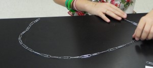
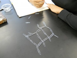
polymer-0235 — Normal polymers are long molecules made up of smaller molecules linked together, much like a paperclip chain.

polymer-0233 — Cross-linked polymers are created when the long chained polymers are linked together by cross-links. It makes for a much sturdier molecule.

To season, you coat the pan with a thin layer of oil and bake it for a while (without anything in it). Baking releases free radicals from the metal that react with the oil to create a cross-linked polymer that’s really hard to break down or wear out, and prevent food from sticking to the pan. Different, cross linked polymers are used in car tires for their durability, but probably not for their lack of stickiness.

Apparently, linseed oil is the best seasoning agent, but it might be a bit hard to find.

Most non-stick, artificial surfaces, are also made of polymers of hydrocarbons, silicon oxides and other interesting chemicals.

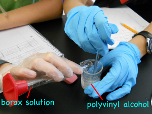
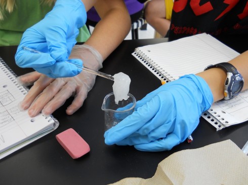
polymer-0251 — Making a cross-linked polymer with borax and polyvinyl alcohol.

In the lab, you can make your own cross-linked polymer “slime” by adding a solution of borax (sodium tetraborate) to a solution of polyvinyl alcohol (1:1 ratio of concentrations) (Practical Chemistry, 2008).

The result is a satisfying goo.

polymer-0254 — Cross-linked polymer "slime".

Media Profanity and Aggression

This research shows that profanity is not harmless. Children exposed to profanity in the media think that such language is ‘normal,’ which may reduce their inhibitions about using profanity themselves. And children who use profanity are more likely to aggress against others.
–Brad Bushman (2011) in a Brigham Young University Press Release.

Exposure to profanity in videogames and on TV appears to affect how teens view and use profanity, and makes them more aggressive. These are the key results of a paper by Sarah Coyne (Coyne et al., 2011). The full article is available online, but is summarized here.

While the first part, at least, of this result might seem obvious — that seeing profanity desensitizes, familiarizes, and leads to increased use — it’s nice to have some scientific corroboration.

The more disturbing result, perhaps, is the link between profanity and aggression. It’s a moderate effect, but the link appears similar to the connection between war games and aggression.

Profanity is kind of like a stepping stone. You don’t go to a movie, hear a bad word, and then go shoot somebody. But when youth both hear and then try profanity out for themselves it can start a downward slide toward more aggressive behavior.
— Sarah Coyne (2011) in a Brigham Young University Press Release.

Sling: A VPython Model Demonstrating Centripetal Force and Conservation of Angular Momentum

sling-anim-500 — Animation captured from the sling.py Vpython model. The yellow arrow shows the centripetal force. The white arrow shows the velocity.

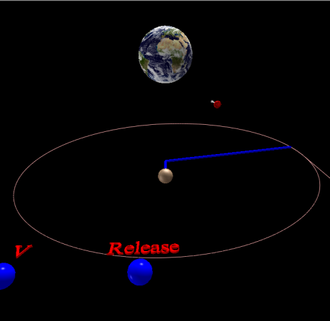
Sitting in a car that’s going around a sharp bend, its easy to feel like there’s a force pushing you against the side of the car. It’s called the centrifugal force, and while it’s real to you as you rotate with the car, if you look at things from the outside (from a frame of reference that’s not rotating) there’s really no force pushing you outward. The only force is the one keeping you in the car; the force of the side of the car on you. This is the centripetal force. Given all the potential for confusion, I created this little VPython model that mimics a sling.

Centripetal Force

In the model, you launch a ball and it goes off in a straight line. That’s inertia. An object will move in a straight line unless there’s some other force acting on it. When the ball hits the string, it catches and the string starts to pull on the ball, taking it away from its straight line trajectory. The force that pulls the ball away from its original straight path is the centripetal force.

centrifA — Image from Stern (2004): (23a) Frames of Reference: The Centrifugal Force

Conservation of Angular Momentum

The ball rotating on the sling has an angular momentum (L) that’s equal to the velocity (v) times its mass (m) times its radius (r) away from the center.

L = mvr , angular momentum

Now, angular momentum is conserved, which means that if you shorten the string, reducing the radius, something else must increase to compensate. Since the mass can’t change, the velocity has to, and the ball speeds up.

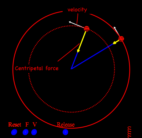
momentum-diag — The ball on the string with the shorter radius has the higher velocity (moves faster). It also has a higher centripetal force. The ball for shortening the radius is not shown in this figure.

I’ve put in a little ball at the end of the string that you can pull on to shorten the radius.

Tangential Velocity

Once the ball is attached to the string, the centripetal force will keep it moving in a circle. If you release the ball then it will fly off in a straight line in whatever direction it was going when you released it. With no forces acting on the ball, inertia says the ball will move in a straight line.

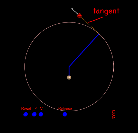
The ball, when released from the string, flies off in a tangent.

To better illustrate the ball’s motion off a tangent, I put in a target to aim for. It’s off the screen for the normal model view, but if you rotate the scene to look due north you’ll see it.

What’s Wrong with Traditional Education

Alison Gopnik points out the people first start to learn by exploration (the same way scientists do), and then learn to do things well by apprenticeship.

When we actually start to look at the fundamentals, it seems children learn by exploring—by experimenting, playing, drawing inferences …. that kind of exploratory learning isn’t just the purview of scientists but seems to be very, very basic. …The other kind of learning that we see, not so much in preschoolers but in school-age children, is what I call guided apprenticeship learning, where you’re not just exploring and finding out new things but learning to perform a skill particularly well.

— Alison Gopnik in Fillion (2011): In conversation: Alison Gopnik in MacLeans.

Kate Fillion’s great interview with Gopnik, a cognitive scientist, is worth the read.

The traditional way of thinking about learning at a university is: there’s somebody who’s a teacher, who actually has some amount of knowledge, and their job is figuring out a way of communicating that knowledge. That’s literally a medieval model; it comes from the days when there weren’t a lot of printed books around, so someone read the book and explained it to everybody else. That’s our model for what university education, and for that matter high school education, ought to be like. It’s not a model that anybody’s ever found any independent evidence for. [my emphasis]

— Alison Gopnik in Fillion (2011): In conversation: Alison Gopnik in MacLeans.

Update

EV, in the comments, recommends Allison Gopnik’s TED talk. It focuses on babies, but is a pretty good presentation.

(via The Dish)

Murmuration: A Flocking of Birds

Amazing footage of an enormous flock of birds in flight by Sophie Windsor Clive.

Murmuration from Sophie Windsor Clive on Vimeo.

Brandon Kelm explains a little of how it works, mostly using terms like “scale-free correlation” and “criticality”, which pretty much sums up that we don’t know a lot about the phenomena.

NetLogo has a nice little Java model showing an attempt at simulating flocking. They give a good description of how there model works.

(via The Dish)

Projectile Motion

Abstract

A series of still photographs of a projectile (soccer ball) in motion were used to determine the equation for the height of the ball (h(t) = 4.9 t² + 14.2 t + 1.25), the initial velocity of the ball (14.2 m), the maximum height of the ball (11.6 m), and the time between each photograph (0.41 s). The problem was solved numerically using MS Excel’s Solver function. There are much easier ways of doing this, which we did not do.

Introduction

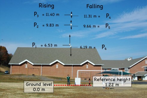
projectile-diagram — Figure 1. Calculated elevation of the soccer ball after launch.

projectile-3832c2-800 — Figure 2. Animation of the soccer ball projectile.

One of physics lab assignments I gave my students was to see if students could use a camera to capture a sequence of images of a projectile, plot the elevation of the projectile from the photographs, determine the constants in the parabolic equation for the height of the projectile, and, in so doing, determine the velocity at which the projectile was launched.

I offered my old, digital Pentax SLR that can take up to seven pictures in quick sequence and be set to fully manual. A digital video camera with a detailed timestamp would have been ideal, but we did not have one available at the time.

Now the easy way of getting the velocity data would be to estimate the heights (h) of the ball from the image using some sort of known reference (in this case the whiteboard), and determine the time between each photograph (Δt) by photographing a stopwatch using the same shutterspeed settings. After all, the average velocity of the ball between two images would be:

$! \bar{v} = \frac{\Delta h}{\Delta t}$

The reference whiteboard is four feet tall (1.22 m) in real life, but 51 pixels tall in the image. Using this ratio (i.e. 1.22 m = 51 px) we can convert the heights of the ball from pixels to meters:

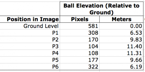
elevations — Table 1. Table showing the conversion of the height of the ball in pixels to elevation (in meters).

Unfortunately, I think my students forgot to do the pictures of the stopwatch to get Δt, the time between each photograph. Since the lab reports are due on Monday, and it’s the weekend now I’m curious to see what they come up with.

However, I was wondering if they could use just the elevation data to back out the Δt. So I gave it a try myself. Even the easiest way of solving this problem is not trivial, in fact, I ended up resorting to Excel’s iterative solver to find the answers. While this procedure probably goes a little beyond what I expect from the typical high school physics student, more advanced students who are taking calculus might benefit.

Procedure

We took the reference whiteboard (1.21 m tall), a soccer ball, and the camera outside. The whiteboard was leant vertically against the post of the soccer goal. The ball was thrown vertically by a student standing next to the whiteboard (see Figure 1) while pictures were taken. The camera’s shutterspeed was 1/250th of a second. The distance from the camera to the person throwing the ball (and to the whiteboard) were not measured.

The procedure was repeated several times, but only one trail was used in this analysis.

The images were loaded onto a computer, and the program GIMP was used to determine the distance, in pixels, from the ground to the projectile. The size of the reference whiteboard, in pixels, was used to calculate the height of the soccer ball in meters.

The elevations measured off the photographs were then used to calculate the release velocity, time between snapshots, and maximum height of the ball.

The Equation for Elevation

I started with the fact that once the ball is released, the only force acting on it is the force of gravity. Since the mass of the ball does not change we only have to consider the acceleration due to gravity (-9.8 m/s²). I also neglect air resistance to make things easier.

Finding the Velocity Equation

Start with the fact that, acceleration is the rate of change of velocity with time. You can write it in the differential form:

$! a = \frac{dv}{dt} = -9.8$

so we integrate with respect to time to get the equation for velocity as a function of time:

$! v(t) = \int -9.8 dt$

$! v(t) = -9.8 t + c$

where c is an unknown constant. What we do know though, is that at the beginning, when the ball is just launched, time is zero (t = 0) so c_v becomes the initial velocity (v₀) at which the ball is thrown:

at t = 0, v(0) = v₀:
$! v_0 = -9.8 (0) + c$

$! v_0 = c$

So our velocity equation becomes:

$! v(t) = -9.8 t + v_0$

Finding the height equation

Now since we know that velocity is the rate of change of distance (in this case height) with time:

$! v(t) = \frac{dh}{dt} = -9.8 t + v_0$

so we integrate again to find the height equation:

$! \frac{dh}{dt} = -9.8 t + v_0$
$! h(t) = \int (-9.8 t + v_0) dt$
$! h(t) = \frac{-9.8 t^2}{2} + v_0 t + c$

Similar to what we did with the velocity equation, to find the new constant c we consider what happens at the start time, when the ball is launched, and t = 0 and h(0) = h₀;

$! h_0 = \frac{-9.8 (0)^2}{2} + v_0 (0) + c$

so:
$! h_0 = c$

The constant is equal to the initial height of the ball — the height of the ball when it’s thrown. So we end up with the final equation:

$! h(t) = \frac{-9.8 t^2}{2} + v_0 t + h_0$

Results

Solving all the unknowns

At this point, although we have an equation for the height of the ball, we don’t know the initial velocity (v₀), nor do we know the initial height of the ball when it’s released (h₀). And we still don’t know the time when the ball is at each position.

With that many unknowns we’d need the same number of independent equations to be able to solve for them all. It may be possible, but instead of analytically solving the equations I opted to take a numerical approach, and use Excel’s Solver function.

I started by setting up the equations to calculate the height of the ball at six different times to correspond with our six height measurements. It was necessary therefore to create a set of variables:

Time when we started taking pictures (t₁): Since we don’t know how long after we threw the ball we started taking pictures, I made this a variable called t₁.
The time between each picture (dt): I made the assumption that the time between each picture would be constant. The shutter speed was constant (1/250th of a second) so there is no obvious reason why the time should be different.
Initial velocity (v₀): The initial upward speed at which the ball was thrown. Obviously, the faster the initial speed the higher the ball goes, so this is a fairly important parameter.
Initial height (h₀): We also don’t precisely know how high the ball was when it was released, so this also needs to be a variable.

By defining the time between each picture as dt, we can write the time that each picture was taken in terms of the time of the initial picture (t₁) and dt. After all the second picture would have been taken dt seconds after the first for a total time of:

$! t(P2) = t_0 + dt$

similarly for all the pictures:

photo-times — Table 2. Table of expressions giving the time when each of the six photos were taken.

Now I set up an Excel spreadsheet and gave all the unknown variable values and initial value of 1:

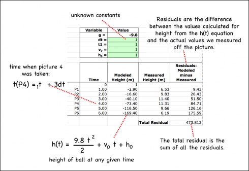
excel-solver — Table 3. Table in Excel for determining the height of a projectile. All of the unknown variables' values are highlighted in green and have been given an initial value of 1.

Now I just had to run Solver and tell it that I wanted the Total Residual, which gives the difference between the h(1) equation’s values for height and the actual, measured values, to be as close to zero as possible. A perfect fit of the equation to the data would have a total residual of one, but that’s not possible when you’re dealing with real data.

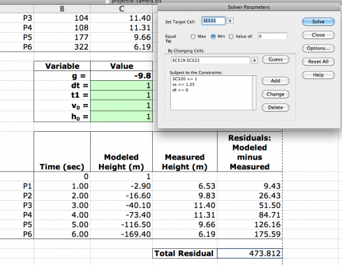
solving — Table 4. Parameters set in Solver to determine the values of the unknown constants.

Even so, I had to goose Solver a bit for it to produce reasonable numbers. I put in a few constraints:

dt >= 0: We could not have a negative time between pictures.
h₀ <= 1.25: 1.25 meters seemed reasonable for the height at which the ball was released.
t₁ <= 1: It also seemed reasonable that the time when the first picture was taken was less than one second after the ball was thrown.

I ran the Solver a few times, and had to reset dt to 0.5 at one point when it had become zero, but the final result looked remarkably good: the total difference between the modeled line and the actual data was only 0.113 meters.

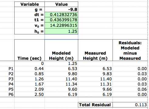
solver-after — Table 5. Solver's solution for the unknown constants in the height equation.

So we found that:

Initial velocity: v₀ = 14.2 m/s
Height at release: h₀ = 1.25 m
Time between pictures: dt = 0.41 s
Time when the first picture was taken: t₁ = 0.44 s

Which makes the height equation:

$! h(t) = \frac{-9.8 t^2}{2} + 14.2 t + 1.25$

Using these constants in the height equation, we could see how good fit the height equation was to the data:

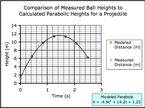
projectile-graph — Figure 3. Graph comparing the modeled heights (from the h(t) equation) to the actual data.

Maximum Height of the Ball

Finally, the maximum height of the ball can be read off the graph, but it can also be determined using the equation for the height of the ball:

$! h(t) = \frac{-9.8 t^2}{2} + v_0 t + h_0$

We know that the maximum height is reached when the ball stops moving upward and starts to descend. At that point, the vertical velocity of the ball is zero. Since the velocity of the ball is the rate of change of height ( $v = \frac{dh}{dt}$ ) we can differentiate the height equation to get an equation for velocity.

$! h(t) = \frac{-9.8 t^2}{2} + v_0 t + h_0$

$! v = \frac{dh}{dt} = -9.8 t + v_0$

since we’ve determined that the initial velocity of the ball is 14.2 m/s we get:

$! v = -9.8 t + 14.2$

when the velocity is zero (v = 0):

$! 0 = -9.8 t + 14.2$

which can be solved for t to find that the time the ball reaches it’s maximum height is:

$! t = 1.45 seconds$

Putting this into the height equation:

$! h(1.45) = \frac{-9.8 (1.45)^2}{2} + 14.2 (1.45) + 1.25$

gives:

$! h_{max} = 11.58 meters$

Discussion

I’m quite happy with the way this project turned out. The fit between the modeled heights (h(t)) and the actual heights was very good.

My primary concern going into the project was that the distortion from the camera lens would make this technique impossible, but that appears not to be a significant problem.

Most of this calculation, including the somewhat tricky numerical solution using Solver could have been avoided if I’d calibrated the camera, simply by pointing it at a stopwatch (using the same shutterspeed as in the experiment) and measuring the time between snapshots. It will therefore be interesting to see if the actual time between shots (dt) is close to the dt of 0.41 seconds calculated by the model.

Finally, as noted above, a video camera with a timestamp would possibly be a more useful technology for this experiment.

Conclusion

It is possible to analyze the projectile path of an object using a series of snapshots, to determine the initial velocity of the projectile, its release height, and the time between snapshots, if you can assume that the time between snapshots is identical. There are, however, much easier methods of solving this problem.

References

None, but this is where they’d be if I had any.

Appendix

The Excel spreadsheet where all the calculations were done is here.

Morning Fog

lake-am-3815c2 — Early morning fog over the lake.

There’s a place on the road to school where you crest a little rise and the St. Albans golf course opens up before you. “Zen-like,” I’ve heard it described. On one lovely fall morning last week the view was absolutely ridiculous. I had to stop.

Resisting the coming winter, warmer air from down south just pushed over the hills overnight, trapping the cooler air in the valley, creating a thermal inversion that trapped a layer of fog just below the tops of the hills. Small tendrils of mist were rising off lake in the bottom of the valley, feeding the fog layer as the cooler valley air condensed the water vapor evaporating off the still warm lake.

Combine the fog, mists, early morning sunlight just beginning to reach into the valley, and the brilliant fall colors contrasting against the still-green lawns, and the result was absolutely amazing.

How the Electoral College Works

The Trouble with the Electoral College

Centripetal Force

Conservation of Angular Momentum

Tangential Velocity

Update

Abstract

Introduction

Procedure

The Equation for Elevation

Finding the Velocity Equation

Finding the height equation

Results

Solving all the unknowns

Maximum Height of the Ball

Discussion

Conclusion

References

Appendix