Elon Musk would like to put his Tesla into Mars orbit. YouTube user ShadowZone shows how it could be done…using Kerbal Space Program. Awesome.
Author: Lensyl Urbano
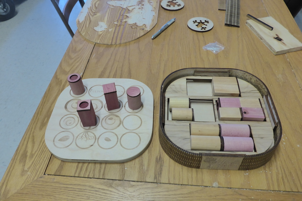
Quarto Set
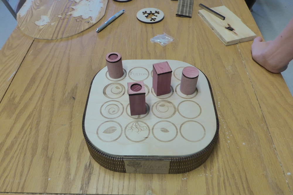
One of the more interesting projects of the last year was the wooden Quarto set I made for our middle schoolers to use during their study hall.
The game is quite an interesting one, as was the build. The pieces (rectangular and cylindrical prisms capped with solid or hollow tops) were fairly simple to make using the table-saw for the bodies and laser cutter for the tops. However, I wanted to make a box for the pieces and have the board with its 4×4 grid of circle serve as the top.
Cutting out the top and bottom of the box out of plywood (on the CNC machine) was easy enough, as was lasering on the grid, but the most fascinating part was making the sides of the box. The rounded corners on the top required rounded sides, so I used the laser to cut a living hinge on a piece of plywood and glued it to the base. Then I used some spacer pieces for the inside to hold up an inset that would hold the pieces.
Cajón
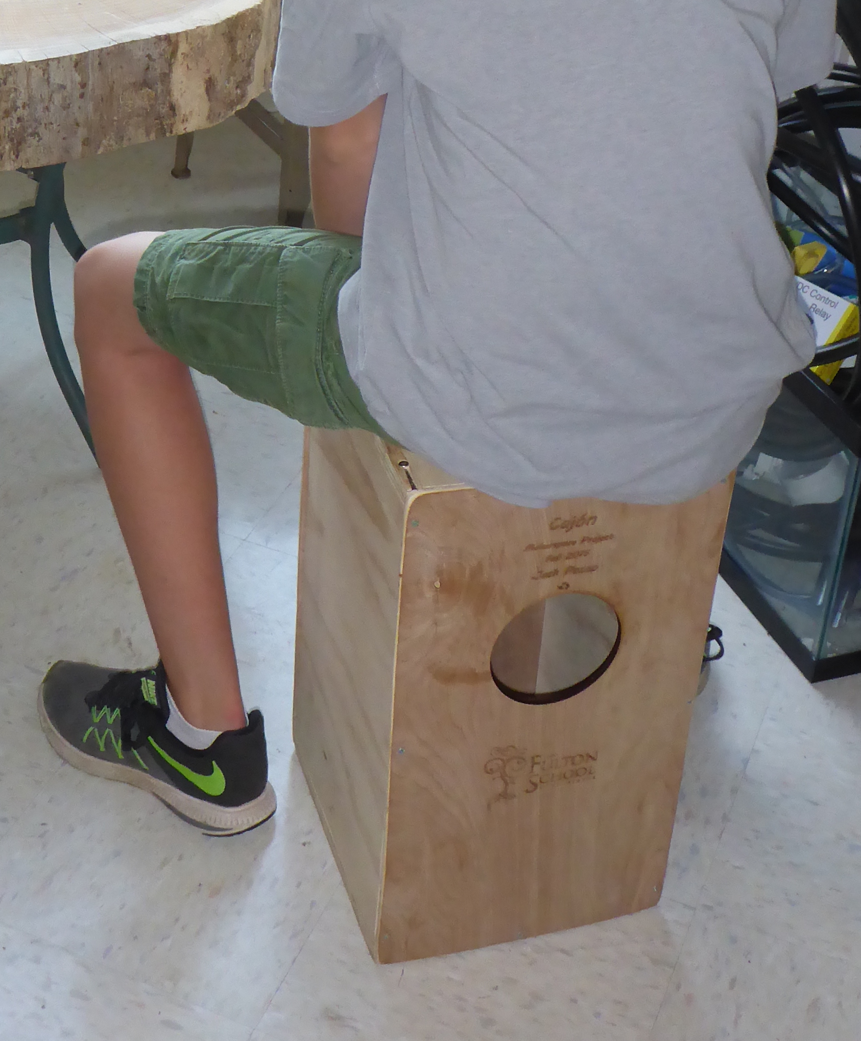
Last year, for an interim project, one of my more musically inclined students decide to build a Cajón. It’s a box shaped drum that you can sit on, with a snare inside. He worked up a simple design in Inkscape and I cut it out on the CNC machine at the Techshop. It turned out quite well, and he even built one that I could keep at school.
Finger Labyrinths

Our first through third grade teachers requested these finger labyrinths. I asked Dr. Steurer to explain how they used them:
Sometimes you just need to be alone. Welcome to our 1-2-3 Classroom “Comfort Zone.” When a child needs a break, they may relax and take a time away from any feeling of pressure or being overwhelmed.
One activity found in the “Comfort Zone” is a finger labyrinth crafted by Dr. Urbano. Children are taught three easy steps for slowly tracing the beautifully designed wooden labyrinth.
Step One: Release – Pause and take a deep breath.
Take a deep breath before you begin your finger walk to the center. This is the time for you to calm yourself and get focused. Let go of everything.
Step Two: Receive – Take in the center.
The center is a place for you to gain calm and peace. You can stay in the center point as long as you need.
Step Three: Return – Slowly take the journey back.
Move back out of the center point. Make the transition from the center back into your daily routine, ready and armed with the experience of peace and calm.
The “Comfort Zone” is one area in our classroom used to support our children in improving their abilities to pay attention, to calm down when they are upset and to make better decisions.
Being Mindful helps with emotional regulation and cognitive focus.
– Dr. Steurer
The Physics of GPS
A nice explanation, from the excellent Real Engineering channel, of the physics of GPS that explains how the satellites must adjust for the effects of special and general relativity.
Generating 3d Terrain

After a lot of hours of experimentation I’ve finally settled on a workable method for generating large-scale 3d terrain.
Data from the NGDC’s Grid Extraction tool. The ETOPO1 (bedrock) option gives topography and bathymetry. You can select a rectangle from a map, but it can’t be too big and, which is quite annoying, you can’t cross the antimeridian.
The ETOPO1 data is downloaded as a GeoTIFF, which can be easily converted to a png (I use ImageMagick convert).

Adjusting the color scale. One interesting property of the data is that it uses a grayscale to represent the elevations that tops out at white at sea-level, then switches to black and starts from there for land (see the above image). While this makes it easy to see the land in the image, it needs to be adjusted to get a good heightmap for the 3d model. So I wrote a python script that uses matplotlib to read in the png image as an array and then I modify the values. I use it to output two images: one of the topography and one of just land and water that I’ll use as a mask later on.

The images I export using matplotlib as grayscale png’s, which can be opened in OpenSCAD using the surface command, and then saved as an stl file. Bigger image files are take longer. A 1000×1000 image will take a few minutes on my computer to save, however the stl file can be imported into 3d software to do with as you will.
Note: H.G. Deitz has a good summary of free tools for Converting Images Into OpenSCAD Models
Bike Silhouette
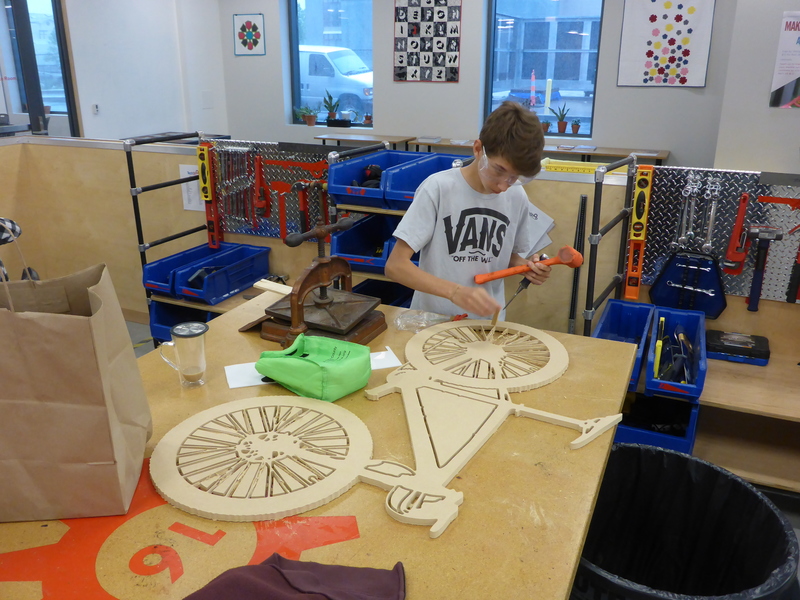
One of my students with a TechShop membership wanted a bike silhouette for a wall hanging. He wanted it to be bigger than he could fit on the laser cutter, so I tried doing it on the CNC router. The problem was that to get the maximum detail we needed to use the smaller drill bits (0.125 inches in diameter), however, after breaking three bits (cheap ones from Harbor Freight) and trying both plywood and MDF, we gave up and just used the larger (0.25 inch) bit. Since the silhouette was fairly large (about 45 inches long), it worked out quite well.
How to Build an 8-bit Computer on a Breadboard
Ben Eater’s excellent series on building a computer from some basic components. It goes how things work from the transistors to latches and flip-flops to the architecture of the main circuits (clock, registers etc). The full playlist.
Other good resources include:
- Nand2Tetris : Building a computer from first principles (this one uses a hardware simulator however): See overview video.