This little embeddable, interactive app uses nth order polynomials to approximate a few curves to demonstrate the Taylor Series.
Author: Lensyl Urbano
Elements by Their Uses
Keith Enevoldsen has an excellent version of the periodic table that has some of the more popular uses of the elements on them.
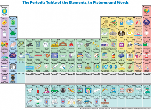
Hat tip to Ms. Douglass for this link.
The Essential Biopolymers
My notes on the four macromolecules that are essential to life as we know it: proteins, fats (lipids), carbohydrates (saccharides), and nucleic acids.


Projectile Paths

I had my Numerical Methods student calculate the angle that would give a ballistic projectile its maximum range, then I had them write a program that did the the same by just trying a bunch of different angles. The diagram above is what they came up with.
It made an interesting pattern that I converted into a face-plate cover for a light switch that I made using the laser at the TechShop.

Maximum Range of a Potato Gun
One of the middle schoolers built a potato gun for his math class. He was looking a the mathematical relationship between the amount of fuel (hair spray) and the hang-time of the potato. To augment this work, I had my Numerical Methods class do the math and create analytical and numerical models of the projectile motion.
One of the things my students had to figure out was what angle would give the maximum range of the projectile? You can figure this out analytically by finding the function for how the horizontal distance (x) changes as the angle (theta) changes (i.e. x(theta)) and then finding the maximum of the function.

Distance as a function of the angle
In a nutshell, to find the distance traveled by the potato we break its initial velocity into its x and y components (vx and vy), use the y component to find the flight time of the projectile (tf), and then use the vx component to find the distance traveled over the flight time.
Starting with the diagram above we can separate the initial velocity of the potato into its two components using basic trigonometry:

 ,
,
so,
 ,
,

Now we know that the height of a projectile (y) is given by the function:

(you can figure this out by assuming that the acceleration due to gravity (a) is constant and acceleration is the second differential of position with respect to time.)
To find the flight time we assume we’re starting with an initial height of zero (y0 = 0), and that the flight ends when the potato hits the ground which is also at zero ((yt = 0), so:


Factoring out t gives:

Looking at the two factors, we can now see that there are two solutions to this problem, which should not be too much of a surprise since the height equation is parabolic (a second order polynomial). The solutions are when:


The first solution is obviously the initial launch time, while the second is going to be the flight time (tf).


You might think it’s odd to have a negative in the equation, but remember, the acceleration is negative so it’ll cancel out.
Now since we’re working with the y component of the velocity vector, the initial velocity in this equation (v0) is really just vy:

so we can substitute in the trig function for vy to get:

Our horizontal distance is simply given by the velocity in the x direction (vx) times the flight time:

which becomes:

and substituting in the trig function for vx (just to make things look more complicated):

and factoring out some of the constants gives:

Now we have distance as a function of the launch angle.
We can simplify this a little by using the double-angle formula:

to get:

Finding the maximum distance
How do we find the maxima for this function. Sketching the curve should be easy enough, but because we know a little calculus we know that the maximum will occur when the first differential is equal to zero. So we differentiate with respect to the angle to get:

and set the differential equal to zero:

and solve to get:


Since we remember that the arccosine of 0 is 90 degrees:


And thus we’ve found the angle that gives the maximum launch distance for a potato gun.
Making Dry-Erase Erasers
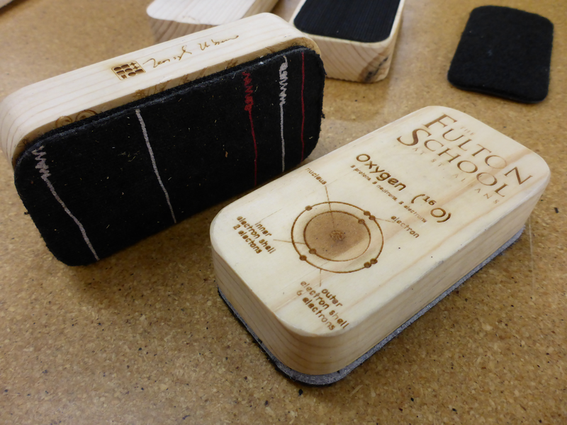
I painted the wall on my new space in the basement to make it a dry-erase surface. Unfortunately, I did not have an eraser to use on it, so, I decided to make my own down at the TechShop. And what started as a simple project turned into a bit of a rabbit hole.
The Shopbot CNC router is great for cutting shapes out of wood. I started with simple rectangular 2 inch by 4 inch blanks with designs and patterns, but that truly does not take advantage of the technological possibilities. Map projections can have some interesting shapes, so I tried a few that I could find black and white vector-graphic maps for on the Wikimedia commons (Mollweide and Sinusoidal projections).
.svg)

After a little sanding (of the edges and sides in particular) I put the wooden blanks on the laser. It helped to cut out a template for the wooden blanks to sit in so I could do multiple blocks at the same time.

I put on a few coats of polyurethane to protect the wood surface (I also tried a spray on sealer I had sitting around–we’ll see which one works better) and then attached velcro strips to the bottom.
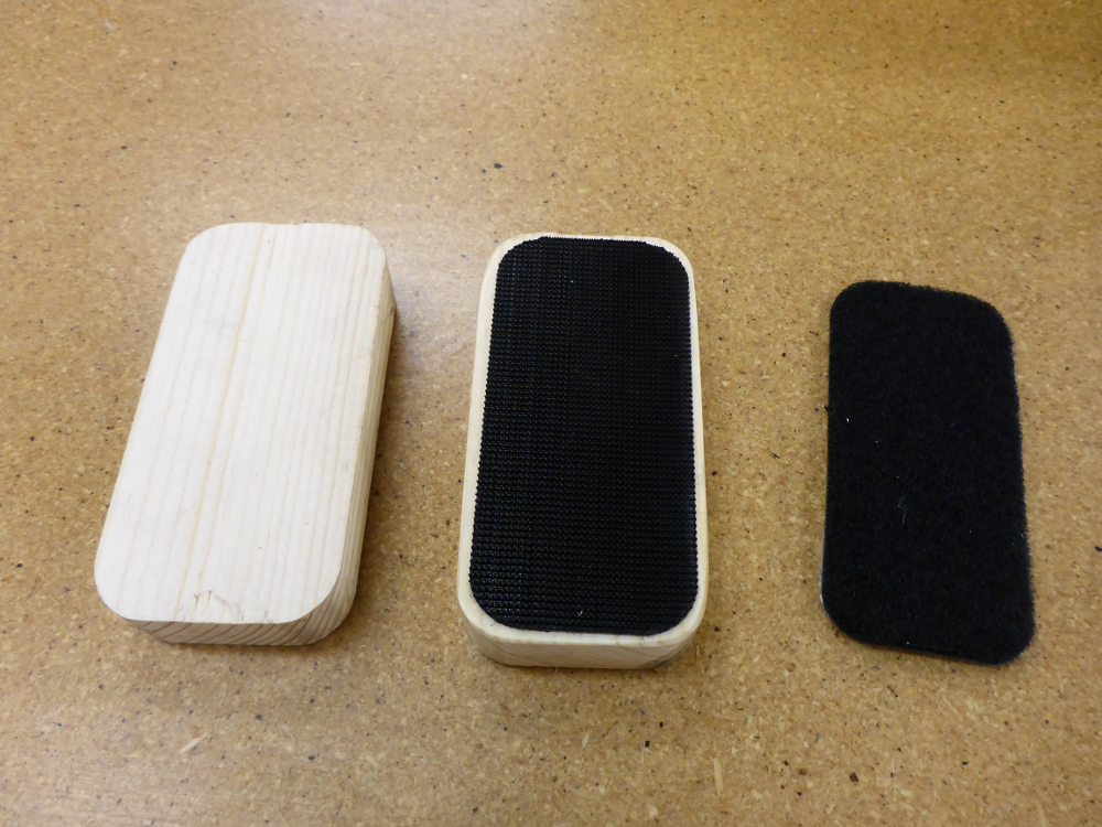
One of my old sweatshirts served as material for the erasing.


TechShop

This September a TechShop branch opened up in St. Louis. I’ve been aware of these neat Makerspaces for a few years now, so it was a pleasant surprise when one turned up in town. Even more surprising (and just as pleasant) was that a parent at our school, who was so excited by the opportunities that a place like the TechShop would offer to a school that tries to emphasize hands-on, experiential education, donated four memberships to the school–one for a faculty member and three for students.
Since there are some age restrictions on which machines minors can use–a lot of the woodshop is off limits until they’re 16 and even then adult supervision is required, I arranged a small application for the student memberships that was only open to middle and high-schoolers. Based on the response I got back, we split the annual memberships by semester, so we have three students using it this fall and three more will have access to them in the spring.
The way the TechShop works is that they have a wide range of equipment under one roof and once you take a safety and basic usage (SBU) class on the particular machine you want to use you can reserve time on the machines. There’s a wood shop with saws, sanders, a lathe, and a CNC machine; a metal shop with the same; a set of 3d printers; a set of laser cutters/etchers; a fabric shop with some serious sowing machines, including one that is computer controlled; an electronics shop; a plastics work area with vacuum forming and injection molding machines. They also do a set of interesting classes on using the design software and some interesting projects that can take advantage of the tools available–I have my eye on the Coptic Bookbinding, and the Wooden Bowl making classes. Finally, they’re set up with classrooms where you can bring students in for small STEAM classes, which includes things like using Arduinos.
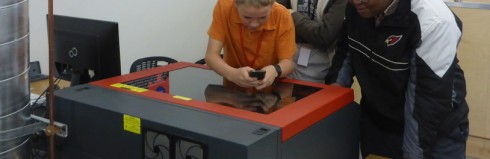
So far, we’ve all taken the Laser class, and there’s just so much that you can do with the laser that we’ve been spending a lot of time experimenting. The students have been etching signs–including a grave marker for our goat MJ who recently passed away–as well as pictures, luggage tags, and making presents. Since this is a machine that the older students can use independently I’ve lost track of everything they’ve been doing.
I’ve also taken the woodshop wood CNC class, so my own experiments have been a bit more expansive, including making dry-erase erasers, floor-holders for quivers for the archery program, simple chemistry molecular model sets (just 2d), boxes for Ms. Fu’s math cards, and I’m trying to figure out how to make a clock.
Sorting algorithms (with Hungarian Dance)
This TedEd video explains a few common sorting methods used in computer science. Sorting can be a challenging computational problem because of the enormous number of comparisons between items that can be involved, so computer scientists has spent a lot of time looking into it.
The video below shows the Quick Sort method using Hungarian folk dance.