Draining a Bottle Part 2: Linearizing Equations when you have to

Yesterday we used calculus to find the equation for the height of water in a large plastic water bottle as the water drained out of a small hole in the bottom.

Perhaps the most crucial point in the procedure was fitting a curve to the measured reduction of the water’s outflow rate over time. Yesterday, in our initial attempt, we used a straight line for the curve, which produced a very good fit.

Figure 1. The change in the outflow rate over time can be well approximated by a straight line.

The R2 value is a measure of how good a fit the data is to the trendline. The straight line gives an R2 value of 0.9854, which is very close to a perfect fit of 1.0 (the lowest R2 can go is 0.0).

The resulting equation, written in terms of the outflow rate (dV/dt) and time (t), was:

 \frac{dV}{dt} = -0.0035 t + 3.9113

However, if you look carefully at the graph in Figure 1, the last few data points suggest that the outflow does not just linearly decrease to zero, but approaches zero asymptotically. As a result, a different type of curve might be a better trendline.

Types of Equations

So my calculus students and I, with a little help from the pre-Calculus class, tried to figure out what types of curves might work. There are quite a few, but we settled for looking at three: a logarithmic function, a reciprocal function, and a square root function. These are shown in Figure 2.

Figure 2. Example curves that might better describe the relationship between outflow and time.

I steered them toward the square root function because then we’d end up with something akin to Torricelli’s Law (which can be derived from the physics). A basic square root function for outflow would look something like this:

 \frac{dV}{dt} = a \sqrt{t} + b

the a coefficient stretches the equation out, while the b coefficient moves the curve up and down.

Fitting the Curve

Having decided on a square-root type function, the next problem was trying to find the actual equation. Previously, we used Excel to find the best fit straight line. However, while Excel can fit log, exponential and power curves, there’s no option for fitting a square-root function to a graph.

To get around this we linearized the square-root function. The equation, after all, looks a lot like the equation of a straight line already, the only difference is the square root of t, so let’s substitute in:

 x = \sqrt{t}

to get:

 \frac{dV}{dt} = a x + b

Now we can get Excel to fit a straight line to our data, but we have to plot the square-root of time versus temperature instead of the just time versus temperature. So we take the square root of all of our time measurements:

Time Square root of time Outflow rate
t (s) t1/2 = x (s1/2) dV/dt (ml/s)
0.0 0 3.91
45.5 6.75 3.52
97.8 9.89 2.94
140.9 11.87 3.52
197 14.04 3.21
257 16.05 3.01
315.1 17.75 2.81
380.1 19.50 2.53
452.9 21.28 2.23
529.6 23.01 1.92
620.7 24.91 1.69
742.7 27.25 1.45

We can now plot the outflow rate versus the square root of time (Figure 3).

Figure 3. Linear trend relating the outflow rate to the square root of time. The regression coefficient (R2) of 0.9948 is better than the simply linear trend of outlfow rate versus time (which was 0.9854).

The equation Excel gives (Figure 3), is:

 \frac{dV}{dt} = -0.1395 x + 5.21

and we can substitute back in for x=t1/2 to get:

 \frac{dV}{dt} = -0.1395 \sqrt{t} + 5.21

Getting back to the Equation for Height

Now we can do the same procedure we did before to find the equation for height.

First we substitute in V=πr2h:

 \frac{d(\pi r^2 h}{dt} = -0.1395 \sqrt{t} + 5.21

Factor out the πr2 and move it to the other side of the equation to solve for the rate of change of height:

 \frac{dh}{dt} = \frac{-0.1395}{\pi r^2} \sqrt{t} + \frac{5.21}{\pi r^2}

Then integrate to find h(t) (remember \sqrt{t} = t^{1/2} ) :

 \int \frac{dh}{dt} dt = \int \left( \frac{-0.1395}{\pi r^2} t^{1/2} + \frac{5.21}{\pi r^2} \right) dt

gives:

 h =  \frac{-0.1395}{(3/2) \pi r^2} t^{3/2} + \frac{5.21}{\pi r^2} t + c

which might look a bit ugly, but that’s only because I haven’t simplified the fractions. Since the radius (r) is 7.5 cm:

 h =  -0.000526 t^{3/2} + 0.029 t + c

Finally we substitute in the initial value (t=0, h=11) to solve for the coefficient:

 c = 11

giving the equation:

 h =  -0.000526 t^{3/2} + 0.029 t + 11

Plotting the equations shows that it matches the measured data fairly well, although not quite as well as when we used the previous linear function for outflow.

Figure 4. Integrating a square root function for the outflow rate gives a modeled function for the changing height over time that slightly undermatches the measured heights.

Discussion

I’m not sure why the square root function for outflow does not give as good a match of the measurements of height as does the linear function, especially since the former better matches the data (it has a better R2 value).

It could be because of the error in the measurements; the gradations on the water bottle were drawn by hand with a sharpie so the error in the height measurements there alone was probably on the order of 2-3 mm. The measurement of the outflow volume in the beaker was also probably off by about 5%.

I suspect, however, that the relatively short time for the experiment (about 15 minutes) may have a large role in determining which model fit better. If we’d run the experiment for longer, so students could measure the long tail as the water height in the bottle got close to the outlet level and the outflow rate really slowed down, then we’d have found a much better match using the square-root function. The linear match of the outflow data produces a quadratic equation when you integrate it. Quadratic equations will drop to a minimum and then rise again, unlike the square-root function which will just continue to sink.

Conclusions

The linearization of the square-root function worked very nicely. It was a great mathematical example even if it did not produce the better result, it was still close enough to be worth it.

Radish Leaf Pesto

In addition to eating the bulbs of the radishes, the leaves are also edible. I heartily endorse Clotilde Dusoulier’s Radish Leaf Pesto. The slight spiciness of the leaves gives it a delightful frisson.

Radish leaf pesto.

Pesto recipes are pretty flexible. I added some fresh cilantro from the garden, some frozen basil leaves, used ground almonds for the nut component, a bit of Manchego for the cheese, and doubled the garlic. I also added a little white wine to reduce the viscosity. I quite liked the end result — we had it on pasta — even if some others though it was a little too adventurous.

The Draining of a Plastic Bottle: Integrating a Physics Experiment into Calculus

Abstract

I punched a small hole (about 1mm radius) in a one gallon plastic bottle and had my students measure the rate at which water drained. Even though the apparatus and measurement technique was fairly rough, we were able to, with a little calculus, determine the equation for the height of the water in the bottle as a function of time.

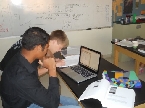
Figure 1. A student uses a stopwatch to measure the outflow rate of water from the plastic bottle.

Introduction

Questions about water draining from a tank are a pretty common in calculus textbooks, but there is a significant difference between seeing the problem written down, and having to figure it out from a physical example. The latter is much more challenging because it does not presuppose any relationships for the change in the height of water with time; students must determine the relationship from the data they collect.

The experimental approach mimics the challenges faced by scientists such as Henry Darcy who first determined the formulas for groundwater flow (Darcy, 1733) almost 300 years ago, not long after the development of modern calculus by Newton and Leibniz (O’Conner and Robertson, 1996).

Procedure

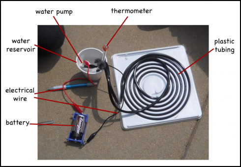
Figure 2. The apparatus.

I punched a small hole, about 1mm in radius, in the base of a plastic, one-gallon bottle. I chose this particular type of bottle because the bulk of it was cylindrical in shape.

Students were instructed to figure out how the rate at which water flowed out (outflow rate) changed with time, and how the height of the water (h) in the bottle changed with time. These relationships would allow me to predict the outflow rate at any time, as well as how much water was left in the container at any time.

Data collection:

  1. To measure height versus time, we marked the side of the bottle (within the cylindrical region) in one centimeter increments and recorded the time it took for the water level to drop from one mark to the next. There were a total of 11 marks.
  2. To measure the outflow rate, we intercepted the outflow using a 25 ml beaker (not shown in Figure 2), and measured the time it took to fill to the 25 ml mark.

Results

Time elapsed since last measurement Height of water in container Time to fill 25ml beaker
Δt (s) h (cm) tf (s)
0.0 11 6.4
45.5 10 7.1
52.3 9 8.5
43.1 8 7.1
56.1 7 7.8
60.6 6 8.3
57.6 5 8.9
65.0 4 9.9
72.8 3 11.2
76.7 2 13.0
91.1 1 14.8
122.0 0 17.3

Table 1: Outflow rate, water height change with time.

To analyze the data, we calculated the total time (the cumulative sum of the elapsed time since the previous measurement) and the outflow rate. The outflow rate is the change in volume with time:

 \text{outflow rate} = \frac{volume}{time} = \frac{dV}{dt} = \frac{25 ml}{t_f}

So our data table becomes:

Time Height of water in container Outflow rate
t (s) h (cm) dV/dt (ml/s)
0.0 11 3.91
45.5 10 3.52
97.8 9 2.94
140.9 8 3.52
197 7 3.21
257 6 3.01
315.1 5 2.81
380.1 4 2.53
452.9 3 2.23
529.6 2 1.92
620.7 1 1.69
742.7 0 1.45

Table 2. Height of water and outflow rate of the bottle.

The graph of the height of the water with time shows a curve, although it is difficult to determine precisely what type of curve. My students started by trying to fit a quadratic equation to it, which should work as we’ll see in a minute.

Figure 3. The decrease in height with time is not a straight line (is non-linear).

The plot of the outflow rate versus time, however, shows a pretty good linear trend. (Note that we do not use the first three datapoints (in Table 2), which we believe are erroneous because we were still sorting out the measuring method.)

Although I’ll note here that the data should ideally be modeled using a square root equation (Torricelli’s Law), that is beyond the present scope of the problem (we’ll try that tomorrow as a follow exercise).

Plotting the data in Excel we could add a linear trendline.

Figure 4. The outflow rate decreases linearly with time.

For the linear trendline, Excel gives the equation:

 y = -0.0035 x + 3.9113

The y-axis is outflow rate (the change in volume with time), and the x axis is time (t), so the linear equation becomes:

 \frac{dV}{dt} = -0.0035 t + 3.9113

Notice that this is a differential equation.

To determine the rate of at which the height of water in the container is changing, we need to recognize that the container is cylindrical in shape, and the volume (V) of a cylinder depends on its radius (r) and height (h):

 V = \pi r^2 h

which can be substituted into differential in the rate equation:

 \frac{d(\pi r^2 h)}{dt} = -0.0035 t + 3.9113

since π and the radius (r) are constants (since the jug’s shape is a cylinder), they can be pulled out of the differential:

 \pi r^2 \frac{dh}{dt} = -0.0035 t + 3.9113

Dividing through by πr2 solves for the rate of change of height:

  \frac{dh}{dt} = \frac{-0.0035 t + 3.9113}{\pi r^2}

Isolating the coefficients gives:

  \frac{dh}{dt} = \frac{-0.0035}{\pi r^2} t + \frac{3.9113}{\pi r^2}

This equation should give the rate at which the height changes with time, however, if you look at it carefully you’ll realize that for the time range we’re using (less than 800 seconds) the value of dh/dt will always be positive. We correct this by recognizing that the outflow rate is a loss of water, so a positive outflow should result in a negative change in height, therefore we rewrite the equation as:

  -\frac{dh}{dt} = \frac{-0.0035}{\pi r^2} t + \frac{3.9113}{\pi r^2}

which gives:

  \frac{dh}{dt} = \frac{0.0035}{\pi r^2} t - \frac{3.9113}{\pi r^2}

Now comes the calculus

Now, we can use this rate equation to find the equation for height versus time by integrating with respect to time:

  \int \frac{dh}{dt} dt = \int \left( \frac{0.0035}{\pi r^2} t - \frac{3.9113}{\pi r^2} \right) dt

to get:

 h = \frac{0.0035}{2 \pi r^2} t^2 - \frac{3.9113}{\pi r^2} t + c

And all we have to do to the find the constant of integration is substitute in a known point, an initial value. As is often the case, the best point to use is the starting point where t=0 makes the rest of the calculations easier. In our case, when t=0, h=11:

 11 = \frac{0.0035}{2 \pi r^2} (0)^2 - \frac{3.9113}{\pi r^2} (0) + c

so:

 c = 11

And our final equation becomes:

 h = \frac{0.0035}{2 \pi r^2} t^2 - \frac{3.9113}{\pi r^2} t + 11

which is a quadratic equation as my students guessed before we did the calculus.

Does it work?

You will notice that in the math above, we never use the height data in determining equation for height versus time; all the calculations are based on the trendline for the outflow rate versus time.

As a result, we can compare the results of our equation to the actual measurements to see if our calculations are even close. Remarkably, they are.

Figure 5. The results from our equation (modeled) match the measured heights so well, the data points are difficult to distinguish on the graph.

Discussion

Despite all the potential for error, particularly, our relatively crude measurement techniques, and the imperfect cylindrical shape of our plastic bottle, the experiment went remarkably well.

Students found it quite challenging, and required some assistance even though this is a problem they have seen before in their textbook.

The problems in the textbook use Torricelli’s Law, which should much better describe the draining of a tank than the linear equation we find for dV/dt.

Torricelli’s Law:

 \frac{dV}{dt} = a \sqrt{2gh}

where a is the area of the outlet hole, and g is the acceleration due to gravity.

In our actual experiment it is difficult to tell that a square root function would work better. Excel does not have an option for matching a square root function, so the calculations would become more involved (although it could be set up using Excel’s iterative solver or Goal Seek function).

Conclusion

Our experiment to use calculus to determine the rate of change of the height of water in a leaking plastic water bottle was a successful exercise even though the roughness of the data collection did not permit identification of the square root law for leakage.

Radishes

Radishes ready for harvest.

The radishes did well this year. Planted in containers on March 29th (in St. Louis, USA), they were harvested one month later. The short, early season means that they’re a workable crop for school. Students can plant, harvest, and consume them all within a semester.

The CDC’s Fruit and Vegetable of the Month website has a little history, some information about the varieties, nutritional information, recipes, and more information about radishes. The University of Illinois Extension also has information about planting and growing.

NutritionData.self.com has some very nice graphical representations of the nutritional value of the food (although their serving size is 1 cup of slices, which seems a bit much).

These sites, however, focus on the radish bulbs, and not on the fact that the leaves are edible. Radish Leaf Pesto is quite good.

Harvested radishes. Both the red bulbs and the green leaves are edible. You'll note that radishes also spot a long tap-root.

Building a Metaphor (Actually a Grill)

The grill entering the final stages of construction by Ryan V. and Robert M.. Photograph by Autumn F.

It took us a little more than half a day to build a grill. It’s a simple thing of cinder blocks and sand, located near the soccer field so it’ll be convenient for bbq’s next year.

It took the highschoolers all morning to dig an outline for the base of the grill and lay in the foundation, despite it being a small, three-quarters of a rectangle shape, and only ten centimeters (4 inches) deep at maximum. The local clay is extremely dense and hard.

The foundations took the longest time to build.

But the foundations were firm, secure, and level.

When the base was done, two middle-schoolers — ably documented by a peer photographer — finished all the visible parts of the structure in just half an hour.

The next day, after I’d given them a presentation on cognitive development during the teenage years that I realized how nice a metaphor the grill construction was for the training of the brain during adolescence. The extensive pruning and myelination that typifies adolescence establish neural pathways are the foundation for future mental growth.

Good, strong, level foundations are the basis for a rich and fulfilling life.

Good foundations require some effort, but they're worth it.

What Computer-Based Learning of Math Should Look Like

Walter Russell Mead (and his commenters) highlight two articles (here and here) on Virginia Tech’s excellent computer-based learning setup for their mathematics classes. Most of the work is done on the computer, either at home or in a shared Math Emporium where teachers are available to help when necessary; which, except for the computer work, is very much like how my class works. It seems close to the ideal way of using technology to allow flexibility in learning and assessment, and is in many ways similar to New York City’s School of One program.

VT’s approach requires some self-motivation on the part of the students — students are able to use the 24 hour a day Emporium at any time — but the model should fit be a good fit for Montessori middle and high-school students who have much independence in managing how they use their time during the day.

Their assessment method also nice as it allows students to pace themselves and take their tests when they’re ready. It is based on students proving that they’ve learned the material — how they learned it is not important, nor is how many practice tests they took before they get to the test.

Each course is broken up into a series of “modules,” available on Emporium computers or the Internet, that students are required to complete within a certain amount of time. Each module outlines a specific set of mathematic principles and concepts. These are translated into specific examples to review and problems to solve.

Once the module materials are completed, students can take randomly generated practice tests that draw on a central bank of thousands of potential questions. If they get questions wrong, the computer refers them back to the appropriate materials, and there’s no limit to the number of practice tests they can take. When they decide they’re ready, students come to the Emporium to take an official, proctored test that’s generated in exactly the same way as the practice quizzes. Then they move to the next module. Instead of marking progress by time—the number of hours spent in proximity to a lecturer—Emporium courses measure advancement by evidence of learning.

— Carey, K., 2008: Transformation 101 in Washington Monthly

Tyler Cowen Walter Russel Mead Ms. Douglass

Pictures from the Royal Society

Knap-weed or matfelon and cornflower or bluebottle, by Richard Waller (1689) from The Royal Society's Picture Library.

The Royal Society’s Picture Library is now available online. It contains images from some of the seminal scientific works of the last four centuries. It’s an excellent resource for teachers and students, who, with registration, can get free high-resolution images for presentations and unpublished theses.

I’m particularly attracted to the biological drawings at the moment because I’m trying to get students to practice their scientific drawing and diagramming.

Control your Destiny: How the Adolescent Brain Works

During your adolescence, which lasts from your early teens into your 20’s, the brain changes rapidly, you develop new abilities and capacities, and the habits of mind and skills you develop will last long into adulthood.

Abilities: The last part of the brain to develop is the Frontal Lobe. It’s responsible for reasoning and judgement — aka Executive Function. So, it’s somewhat understandable that teens often have poor impulse control — their Frontal Lobe (the prefrontal cortex in particular) is still developing.

The parts of the adolescent brain.

However that’s not an excuse. It is essential for adolescents to be held to account, because it’s only by practicing responsibility that they get to learn how to use their Executive thinking skills.

Because that’s how we learn — by practicing.

When we’re learning something new, brain cells, called neurons, reach out and connect to form networks. As we practice and focus on specific things — certain patterns of movement or certain ways of thought — some of the unused connections get pruned away, while others become stronger. The axons that connect the most-used pathways get coated in myelin, which acts as an insulator to make sure signals can pass quickly and efficiently.

Neurons in the brain transmit information to each other along long axons and across the synaptic gap.

By reorganizing the connections between brain cells, the brain learns and becomes better at what you’re practicing. Thus we gradually transition from novices to experts.

However, there is a cost.

Making strong pathways makes for quicker thinking about the things we’ve practiced, but makes our brains somewhat less flexible at learning new things. We develop habits of mind that stay with us for a long time.

Some of those habits we might not actually want to keep; and there’s also the possibility that we might not develop some habits of mind that we really would like to have.

The development of the frontal lobe during adolescence opens a window of opportunity for learning good judgement/executive function, but it does not mean we actually will learn it. We need to actually practice it.

So, if you would like to know yourself, want to be able to control yourself, and, especially, want to shape the future person you will become, then you’re going to have to figure out: which habits of mind you want to be practicing and which ones you don’t.