Key to it is the Modified Newtonian Dynamics (MOND) equation to explain why the stars at the outer edges of galaxies are moving faster than Newton’s force law predicts they should be.
Velocities of stars further away from the center of the galactic disk (larger R) have a higher velocity (V) than predicted by Newtonian physics. Dark matter has been used to explain this discrepancy, but tweaking the physics equations could do so as well. Image from Wikipedia.
Newton’s Second Law, finds that the Force (F) acting on an object is equal its mass (m) multiplied by its acceleration (a).
The MOND equation adjusts this by adding in another multiplication factor (μ)
μ is just really close to 1 under “normal” everyday conditions, but gets bigger when accelerations are really, really small. Based on the evidence so far an equation for μ may be:
where, a₀ is a really, really small acceleration.
Factoring this μ factor into the equation for the force due to gravity () changes it from:
into:
The key point is that in the first term, which is our standard version, the denominator is the radius squared () while the second term has a plain radius denominator ().
This means as the distance between two objects gets larger, the first term decreases much faster and the second term becomes more important.
As a result, the gravitational pull between, say a star at the edge of a galaxy and the center of the galaxy, is not as small as the standard gravitational equation would predict it would be, and the stars a the edge of galaxies move faster than they would be predicted to be without the additional term.
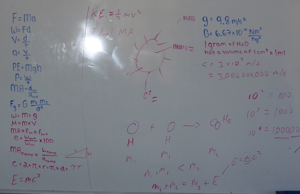
Part of physical science for the middle school is to start going beyond the conceptual, and making the connection between equations in science and algebra. So, we’ve started making note cards for the numerous laws we’ve encountered so far.
The post below was contributed by Michael Schmidt, our math teacher.
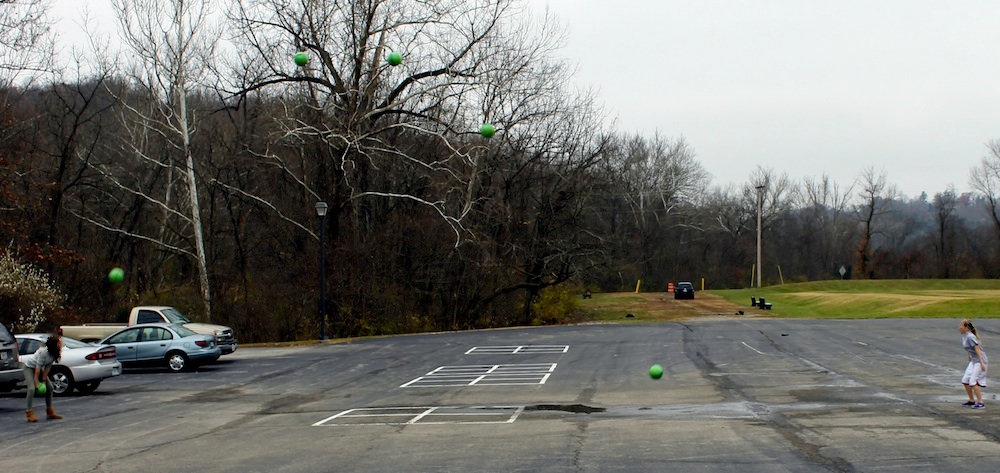
Layered image showing the ballistic path of the green ball thrown by two middle school students. Image by Michael Schmidt.
Parabolas can be a daunting new subject for some students. Often students are not aware of why a parabola may be useful. Luckily, nature always has an answer. Most children realize that a ball thrown through the air will fallow a particular arch but few have made the connected this arch to a parabola. Wonderfully, with a little technology this connection can be made.
With Ms. Hahn’s Canon SLR, I had some of my students throw a ball around outside and took a series of quick pictures of the ball in flight. Since my hand is not very steady, I took the pictures and used the Hugin’s image_stack_align program to align each photo so I could stack them in GIMP.
Within GIMP, I layered the photos on top of each other and cut out the ball from each layer then composed those onto one image. Careful not to move the ball since our later analysis will be less accurate. The result will look something like the following:
Now that there is an image for student to see, we can determine the ball’s height at each point using their own height as a reference. We can then use this information to model a parabola to the data with a site like: http://www.arachnoid.com/polysolve/ .
For the more advanced student an investigation of the least-squares algorithm used by the site may be done.
Now, once we have an expression for the parabola, students can compare how fast they sent the ball into the air.
A ball rolling down a ramp hits a car which moves off uphill. Can you come up with an experiment to predict how far the car will move if the ball is released from any height? What if different masses of balls are used?
Students try to figure out the relationship between the ball's release height and how far the car moves.
For my middle school class, who’ve been dealing with linear relationships all year, they could do this easily if the distance the car moves is directly proportional to height from which the ball was released?
The question ultimately comes down to momentum, but I really didn’t know if the experiment would work out to be a nice linear relationship. If you do the math, you’ll find that release height and the maximum distance the car moves are directly proportional if the momentum transferred to the car by the ball is also directly proportional to the velocity at impact. Given that wooden ball and hard plastic car would probably have a very elastic collision I figured there would be a good chance that this would be the case and the experiment would work.
It worked did well enough. Not perfectly, but well enough.
Yesterday we used calculus to find the equation for the height of water in a large plastic water bottle as the water drained out of a small hole in the bottom.
Perhaps the most crucial point in the procedure was fitting a curve to the measured reduction of the water’s outflow rate over time. Yesterday, in our initial attempt, we used a straight line for the curve, which produced a very good fit.
Figure 1. The change in the outflow rate over time can be well approximated by a straight line.
The R2 value is a measure of how good a fit the data is to the trendline. The straight line gives an R2 value of 0.9854, which is very close to a perfect fit of 1.0 (the lowest R2 can go is 0.0).
The resulting equation, written in terms of the outflow rate (dV/dt) and time (t), was:
However, if you look carefully at the graph in Figure 1, the last few data points suggest that the outflow does not just linearly decrease to zero, but approaches zero asymptotically. As a result, a different type of curve might be a better trendline.
Types of Equations
So my calculus students and I, with a little help from the pre-Calculus class, tried to figure out what types of curves might work. There are quite a few, but we settled for looking at three: a logarithmic function, a reciprocal function, and a square root function. These are shown in Figure 2.
Figure 2. Example curves that might better describe the relationship between outflow and time.
I steered them toward the square root function because then we’d end up with something akin to Torricelli’s Law (which can be derived from the physics). A basic square root function for outflow would look something like this:
the a coefficient stretches the equation out, while the b coefficient moves the curve up and down.
Fitting the Curve
Having decided on a square-root type function, the next problem was trying to find the actual equation. Previously, we used Excel to find the best fit straight line. However, while Excel can fit log, exponential and power curves, there’s no option for fitting a square-root function to a graph.
To get around this we linearized the square-root function. The equation, after all, looks a lot like the equation of a straight line already, the only difference is the square root of t, so let’s substitute in:
to get:
Now we can get Excel to fit a straight line to our data, but we have to plot the square-root of time versus temperature instead of the just time versus temperature. So we take the square root of all of our time measurements:
Time
Square root of time
Outflow rate
t (s)
t1/2 = x (s1/2)
dV/dt (ml/s)
0.0
0
3.91
45.5
6.75
3.52
97.8
9.89
2.94
140.9
11.87
3.52
197
14.04
3.21
257
16.05
3.01
315.1
17.75
2.81
380.1
19.50
2.53
452.9
21.28
2.23
529.6
23.01
1.92
620.7
24.91
1.69
742.7
27.25
1.45
We can now plot the outflow rate versus the square root of time (Figure 3).
Figure 3. Linear trend relating the outflow rate to the square root of time. The regression coefficient (R2) of 0.9948 is better than the simply linear trend of outlfow rate versus time (which was 0.9854).
The equation Excel gives (Figure 3), is:
and we can substitute back in for x=t1/2 to get:
Getting back to the Equation for Height
Now we can do the same procedure we did before to find the equation for height.
First we substitute in V=πr2h:
Factor out the πr2 and move it to the other side of the equation to solve for the rate of change of height:
Then integrate to find h(t) (remember) :
gives:
which might look a bit ugly, but that’s only because I haven’t simplified the fractions. Since the radius (r) is 7.5 cm:
Finally we substitute in the initial value (t=0, h=11) to solve for the coefficient:
giving the equation:
Plotting the equations shows that it matches the measured data fairly well, although not quite as well as when we used the previous linear function for outflow.
Figure 4. Integrating a square root function for the outflow rate gives a modeled function for the changing height over time that slightly undermatches the measured heights.
Discussion
I’m not sure why the square root function for outflow does not give as good a match of the measurements of height as does the linear function, especially since the former better matches the data (it has a better R2 value).
It could be because of the error in the measurements; the gradations on the water bottle were drawn by hand with a sharpie so the error in the height measurements there alone was probably on the order of 2-3 mm. The measurement of the outflow volume in the beaker was also probably off by about 5%.
I suspect, however, that the relatively short time for the experiment (about 15 minutes) may have a large role in determining which model fit better. If we’d run the experiment for longer, so students could measure the long tail as the water height in the bottle got close to the outlet level and the outflow rate really slowed down, then we’d have found a much better match using the square-root function. The linear match of the outflow data produces a quadratic equation when you integrate it. Quadratic equations will drop to a minimum and then rise again, unlike the square-root function which will just continue to sink.
Conclusions
The linearization of the square-root function worked very nicely. It was a great mathematical example even if it did not produce the better result, it was still close enough to be worth it.
I punched a small hole (about 1mm radius) in a one gallon plastic bottle and had my students measure the rate at which water drained. Even though the apparatus and measurement technique was fairly rough, we were able to, with a little calculus, determine the equation for the height of the water in the bottle as a function of time.
Figure 1. A student uses a stopwatch to measure the outflow rate of water from the plastic bottle.
Introduction
Questions about water draining from a tank are a pretty common in calculus textbooks, but there is a significant difference between seeing the problem written down, and having to figure it out from a physical example. The latter is much more challenging because it does not presuppose any relationships for the change in the height of water with time; students must determine the relationship from the data they collect.
The experimental approach mimics the challenges faced by scientists such as Henry Darcy who first determined the formulas for groundwater flow (Darcy, 1733) almost 300 years ago, not long after the development of modern calculus by Newton and Leibniz (O’Conner and Robertson, 1996).
Procedure
Figure 2. The apparatus.
I punched a small hole, about 1mm in radius, in the base of a plastic, one-gallon bottle. I chose this particular type of bottle because the bulk of it was cylindrical in shape.
Students were instructed to figure out how the rate at which water flowed out (outflow rate) changed with time, and how the height of the water (h) in the bottle changed with time. These relationships would allow me to predict the outflow rate at any time, as well as how much water was left in the container at any time.
Data collection:
To measure height versus time, we marked the side of the bottle (within the cylindrical region) in one centimeter increments and recorded the time it took for the water level to drop from one mark to the next. There were a total of 11 marks.
To measure the outflow rate, we intercepted the outflow using a 25 ml beaker (not shown in Figure 2), and measured the time it took to fill to the 25 ml mark.
Results
Time elapsed since last measurement
Height of water in container
Time to fill 25ml beaker
Δt (s)
h (cm)
tf (s)
0.0
11
6.4
45.5
10
7.1
52.3
9
8.5
43.1
8
7.1
56.1
7
7.8
60.6
6
8.3
57.6
5
8.9
65.0
4
9.9
72.8
3
11.2
76.7
2
13.0
91.1
1
14.8
122.0
0
17.3
Table 1: Outflow rate, water height change with time.
To analyze the data, we calculated the total time (the cumulative sum of the elapsed time since the previous measurement) and the outflow rate. The outflow rate is the change in volume with time:
So our data table becomes:
Time
Height of water in container
Outflow rate
t (s)
h (cm)
dV/dt (ml/s)
0.0
11
3.91
45.5
10
3.52
97.8
9
2.94
140.9
8
3.52
197
7
3.21
257
6
3.01
315.1
5
2.81
380.1
4
2.53
452.9
3
2.23
529.6
2
1.92
620.7
1
1.69
742.7
0
1.45
Table 2. Height of water and outflow rate of the bottle.
The graph of the height of the water with time shows a curve, although it is difficult to determine precisely what type of curve. My students started by trying to fit a quadratic equation to it, which should work as we’ll see in a minute.
Figure 3. The decrease in height with time is not a straight line (is non-linear).
The plot of the outflow rate versus time, however, shows a pretty good linear trend. (Note that we do not use the first three datapoints (in Table 2), which we believe are erroneous because we were still sorting out the measuring method.)
Although I’ll note here that the data should ideally be modeled using a square root equation (Torricelli’s Law), that is beyond the present scope of the problem (we’ll try that tomorrow as a follow exercise).
Plotting the data in Excel we could add a linear trendline.
Figure 4. The outflow rate decreases linearly with time.
For the linear trendline, Excel gives the equation:
The y-axis is outflow rate (the change in volume with time), and the x axis is time (t), so the linear equation becomes:
Notice that this is a differential equation.
To determine the rate of at which the height of water in the container is changing, we need to recognize that the container is cylindrical in shape, and the volume (V) of a cylinder depends on its radius (r) and height (h):
which can be substituted into differential in the rate equation:
since π and the radius (r) are constants (since the jug’s shape is a cylinder), they can be pulled out of the differential:
Dividing through by πr2 solves for the rate of change of height:
Isolating the coefficients gives:
This equation should give the rate at which the height changes with time, however, if you look at it carefully you’ll realize that for the time range we’re using (less than 800 seconds) the value of dh/dt will always be positive. We correct this by recognizing that the outflow rate is a loss of water, so a positive outflow should result in a negative change in height, therefore we rewrite the equation as:
which gives:
Now comes the calculus
Now, we can use this rate equation to find the equation for height versus time by integrating with respect to time:
to get:
And all we have to do to the find the constant of integration is substitute in a known point, an initial value. As is often the case, the best point to use is the starting point where t=0 makes the rest of the calculations easier. In our case, when t=0, h=11:
so:
And our final equation becomes:
which is a quadratic equation as my students guessed before we did the calculus.
Does it work?
You will notice that in the math above, we never use the height data in determining equation for height versus time; all the calculations are based on the trendline for the outflow rate versus time.
As a result, we can compare the results of our equation to the actual measurements to see if our calculations are even close. Remarkably, they are.
Figure 5. The results from our equation (modeled) match the measured heights so well, the data points are difficult to distinguish on the graph.
Discussion
Despite all the potential for error, particularly, our relatively crude measurement techniques, and the imperfect cylindrical shape of our plastic bottle, the experiment went remarkably well.
Students found it quite challenging, and required some assistance even though this is a problem they have seen before in their textbook.
The problems in the textbook use Torricelli’s Law, which should much better describe the draining of a tank than the linear equation we find for dV/dt.
Torricelli’s Law:
where a is the area of the outlet hole, and g is the acceleration due to gravity.
In our actual experiment it is difficult to tell that a square root function would work better. Excel does not have an option for matching a square root function, so the calculations would become more involved (although it could be set up using Excel’s iterative solver or Goal Seek function).
Conclusion
Our experiment to use calculus to determine the rate of change of the height of water in a leaking plastic water bottle was a successful exercise even though the roughness of the data collection did not permit identification of the square root law for leakage.


 ) changes it from:

 ) while the second term has a plain radius denominator (
 ).
).


")


 ) :
) :


