Here’s another attempt to create embeddable graphs of mathematical functions. This one allows users to enter the equation in text form, has the option to enter the domain of the function, and expects there to be multiple functions plotted at the same time. Instead of writing the plotting functions myself I used the FLOT plotting library.
Category: Mathematics
A Concept Map for Mathematical Functions
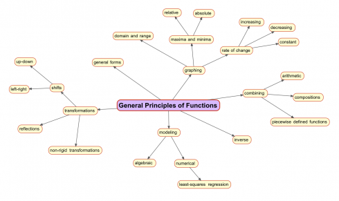
This year I’m trying teaching pre-Calculus (and it should work for some parts of algebra as well) based on this concept map to use as a general way of looking at functions. Each different type of function can by analyzed by adapting the map. So linear functions should look like this:
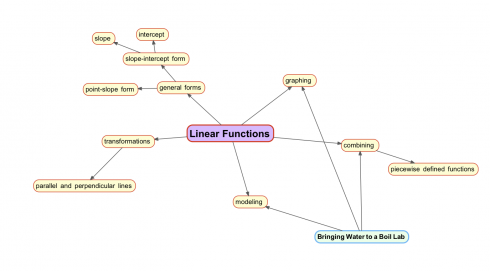
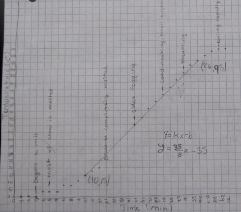
You’ll note the bringing water to a boil lab at the bottom left. It’s an adaptation of the melting snow lab my middle schoolers did. For the study of linear equations we’ll define the function using piecewise defined functions.
Understanding the Extinction of the Dinosaurs (and the Survival of Mammals)
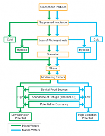
This neat paper (Robertson et al., 2013) in the Journal of Geophysical Research makes an interesting attempt to explain the pattern of extinctions that occurred at the end of the Cretaceous: why most of the dinosaurs died out, and why ocean organisms were more severely affected than freshwater organisms by the long winter after the asteroid impact.
The flow chart explains:
They also include an interesting figure showing how long an organism might survive based on how large it is, which I may be able to use in pre-Calculus when we’re discussing log scales and linearizing equations.
![Allometric relationship between body size and time to death by starvation for multicellular poikilotherms in the absence of food (red, drawn from the equation of Peters [1983, p. 42]). Names of various types of organisms are shown as an indication of body size. Image and caption from Robertson et al., 2013.](http://MontessoriMuddle.org/wp-content/uploads/2013/07/Robertson_et_al_2013_Fig1-490x381.png)
The article is written well enough that an interested high school biology student should be able to decipher (and present) it.
How to be Lucky
The lucky try more things, and fail more often, but when they fail they shrug it off and try something else. Occasionally, things work out.
— McRaney, 2013: Survivorship Bias on You Are Not So Smart.
David McRaney synthesizes work on luck in an article on survivorship bias.
… the people who considered themselves lucky, and who then did actually demonstrate luck was on their side over the course of a decade, tended to place themselves into situations where anything could happen more often and thus exposed themselves to more random chance than did unlucky people.
Unlucky people are narrowly focused, [Wiseman] observed. They crave security and tend to be more anxious, and instead of wading into the sea of random chance open to what may come, they remain fixated on controlling the situation, on seeking a specific goal. As a result, they miss out on the thousands of opportunities that may float by. Lucky people tend to constantly change routines and seek out new experiences.
McRaney goes also points out how this survivorship bias negatively affects scientific publications (scientists tend to get successful studies published but not ones that show how things don’t work), and in war (deciding where to armor airplanes).
What are the odds?
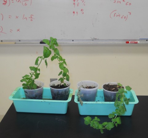
My middle school class stumbled upon a nice probability problem that I might just use in my pre-calculus exam.
Oregano
You see, four of my students took cuttings of oregano plants from the pre-school herb gardens when we were studying asexual reproduction, but only three of them grew roots.
That gives a 75% success rate.
![]()
The next time I do it, however, I want each student to have some success. If I have them take two cuttings that should increase the chances that at least plant will grow. And we can quantify this.
If the probability of success for each cutting is 75% then the probability of failure is 25%.
P[failure] = 0.25
Given a probability of one plant failing of 25%, the probability of both plants failing is the probability of one plant failing and the other plant failing, which, mathematically, is:
P[2 failures] = P[failure] x P[failure]
P[2 failures] = 0.25 x 0.25
P[2 failures] = 0.252
P[2 failures] = 0.0625
So the probability of at least one plant growing is the opposite of the probability of two failures:
P[at least 1 success of two plants] = 1 – P[2 failures]
P[at least 1 success of two plants] = 1 – 0.0625
P[at least 1 success of two plants] = 0.9375
which is about 94%.
If I had the students plant three cuttings instead, then the probability of at least one success would be:
P[at least 1 success of 3 plants] = 1 – P[3 failures]
P[at least 1 success of 3 plants] = 1 – 0.253
P[at least 1 success of 3 plants] = 1 – 0.02
P[at least 1 success of 3 plants] = 0.98
So 98%.
This means that if I had a class of 100 students then I would expect only two students to not have any cuttings grow roots.
An Equation
In fact, from the work I’ve done here, I can write an equation linking the number of cuttings (let’s call this n) and the probability of success (P). I did this with my pre-calculus class today:
![]()
so if each student tries 4 cuttings, the probability of success is:
P = 1 – 0.254
P = 1 – 0.004
P = 0.996
Which is 96.6%, which would make me pretty confident that at least one will grow roots.
However, what if I knew the probability of success I needed and then wanted to back calculate the number of plants I’d need to achieve that probability, I could rewrite the equation solving for n:
Start with:
![]()
isolate the term with n by moving it to the other side of the equation, and switching P as well:
![]()
take the natural log of both sides (we could take the log to the base 10 if we wanted, or any other base log, but ln should work just as well).
![]()
now use the rules of logarithms to bring the exponent down into a multiplication:
![]()
solving for n gives:
![]()
Note that the probability has to be given as a fraction (between 0 and 1), so 90% is P = 0.9. A few of my students made that mistake.
Lavender

At the same time my students were making oregano cuttings, six of them were making cuttings of lavender. Only one of the cuttings grew.
So now I need to find out how many lavender cuttings each student will have to make for me to be 90% sure that at least one of their cuttings will grow roots.
Students can do the math (either by doing the calculations for each step, or by writing and solving the exponential equation you can deduce from the description above), but the graph below shows the results:

Basic JavaScript
- Basic Webpage template (using Jquery): basic-jquery.zip
One of my students couldn’t get VPython to install and run her computer. She was running Windows 8, and I have not used Windows, much less this version of it to figure out what the problem was. This is one of the challenges with a bring your own device policy. So, instead I gave the lesson on numerical integration using javascript.
To make things easier, I create a barebones template of a webpage build around javascript (using the jquery library to make interactivity easier).
If you open the webpage file (index.html) in your browser you should see nothing but the word “Hello”. The template is blank, but it’s ready so students can start with the javascript programming right away, which a few of my programming elective students have done.
For reference, this file (basic-jquery-numeric-int.zip) uses the template to create a program that does numerical integration. Someone using the webpage can enter the limits (a and b) and the number of trapezoids to use (n), and the program calculates calculates the area under the curve f(x) = -x2/4 + x + 4.
It’s a very bare template and doesn’t have any comments, so it’s not useful unless you’re at least a little familiar with html and javascript and just need a clean place to start.
Programming Numerical Integration with Python (and Javascript)
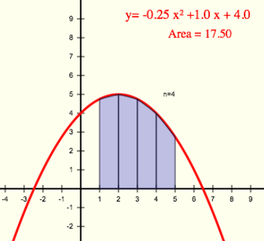
I gave a quick introduction to programming for my calculus class, which has been working on numerical integration.
Numerical integration is usually used for functions that can’t be integrated (or not easily integrated) but for this example we’ll use a simple parabolic function so we can compare the numerical results to the analytical solution (as seen here).
With the equation:
![]()
To find the area under the curve between x = 1 and x = 5 we’d find the definite integral:
![]()
which gives the result:
![]()
For numerical integration, we break the area of concern into a number of trapezoids, find the areas of all the trapezoids and add them up.
We’ll define the left and right boundaries of the area as a and b, and we can write the integral as:
![]()

We also have to choose a number of trapezoids (n) or the width of each trapezoid (dx). Here we choose four trapezoids (n = 4), which gives a trapezoid width of one (dx = 1).

So if we define the x values of the left and right sides of the first trapezoids as x0 and x1, the area of the first trapezoid is:
![]()
For this program, we’ll set the trapezoid width (dx) and then calculate the number of trapezoids (n) based on the width and the locations of the end boundaries a and b. So:
![]()
and the sum of all the areas will be:
![]()
We can also figure out that since the x values change by the same value (dx) for every trapezoid, it’s an arithmetic progression, so:
![]()
and,
![]()
so our summation becomes:
![]()
Which we can program with:
numerical_integration.py
# the function to be integrated
def func(x):
    return -0.25*x**2 + x + 4

# define variables
a = 1.          # left boundary of area
b = 5.          # right boundary of area
dx = 1          # width of the trapezoids

# calculate the number of trapezoids
n = int((b - a) / dx)

# define the variable for area
Area = 0

# loop to calculate the area of each trapezoid and sum.
for i in range(1, n+1):
    #the x locations of the left and right side of each trapezpoid
    x0 = a+(i-1)*dx
    x1 = a+i*dx

    #the area of each trapezoid
    Ai = dx * (func(x0) + func(x1))/ 2.

    # cumulatively sum the areas
    Area = Area + Ai

#print out the result.
print "Area = ", Area
And the output looks like
>>>
Area =  17.5
>>>
While the programming is pretty straightforward, it was a bit of a pain getting Python to work for one of my students who is running Windows 8. I still have not figured out a way to get it to work properly, so I’m considering trying to do it using Javascript.
Update
The javascript functions for numerical integration:
function numerically_integrate(a, b, dx, f) {

	// calculate the number of trapezoids
	n = (b - a) / dx;

	// define the variable for area
	Area = 0;

	//loop to calculate the area of each trapezoid and sum.
	for (i = 1; i <= n; i++) {
		//the x locations of the left and right side of each trapezpoid
		x0 = a + (i-1)*dx;
		x1 = a + i*dx;

		// the area of each trapezoid
		Ai = dx * (f(x0) + f(x1))/ 2.;

		// cumulatively sum the areas
		Area = Area + Ai

	}
	return Area;
}

//define function to be integrated
function f(x){
	return -0.25*Math.pow(x,2) + x + 4;
}

// define variables
a = 1;		// left boundary of area
b = 5;		// right boundary of area
dx = 1;		// width of the trapezoids

// print out output
alert("Area = "+ numerically_integrate(a, b, dx, f));
This is a demonstration of a full html file that uses the function, and should work in any modern browser (download files: numerical-integration.zip).
Update 2
I’ve added the above javascript code to the embeddable graphs to allow it to calculate and display numerical integrals: you can change the values in the interactive graph below.
Profits per Explosion: An application of Linear Regression
[Michael Bay] earns approximately 3.2 million $ for every explosion in his movies and a Michael Bay movie without explosions would earn 154.4 million $. This means that if Michael Bay wants to make a movie that earns more than Avatar’s 2781.5 million $ he has to have 817 explosions in his movie.
— Reddit:User:Mike-Dane: Math and Movies on Imgur.com.
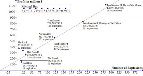
Reddit user Mike-Dane put together these entertaining linear regressions of a couple directors’ movie statistics. They’re a great way of showing algebra, pre-algebra, and pre-calculus students how to interpret graphs, and a somewhat whimsical way of showing how math can be applied to the fields of art and business.
Linear regression matches the best fit straight-line equations to data. The general equation for a straight line is:
y = mx + b
where m is the slope of the line — how fast in increases or decreases == and b is the intercept on the y-axis — which gives the initial value of the function.
So, for example, the Micheal Bay, profits vs. explosions, linear equation is:
Profit (in $millions) = 3.2 × (# of explosions) + 154
which means that a Michael Bay movie with no explosions (where # of explosions= 0) would make $154 million. And every additional explosion in a movie adds $3.2 million to the profits.
Furthermore, the regression coefficient (R2) of 0.89 shows that this equation is a pretty good match to the data.
Mike-Dane gets an even better regression coefficient (R2 = 0.97) when he compares the quality of M. Night Shyamalan over time.
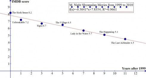
In this graph the linear regression equation is:
Movie Score = -0.3014 × (year after 1999) + 7.8354
This equations suggests that the quality of Shyamalan’s movies decreases (notice the negative sign in the equation) by 0.3014 points every year. If you wanted to, you could, using some basic algebra, determine when he’d score a 0.