Introducing Polynomials

If you recall, straight lines have a general equation that looks like this:

$y=mx+b$ (1)

This is called the slope-intercept form of the equation, because m gives the slope, and b tells where the line intercepts the y-axis. For example the line:

$y=2x-3$ (2)

looks like:

Now, in the slope-intercept form, m and b represent numbers. In our example, m = 2 and b = 3.

So what if, instead of calling them m and b we used the same letter (let’s use a) and just gave two different subscripts so:

$m = a_1$ and,
$b = a_0$

therefore equation (1):

$y=mx+b$

becomes:
$y = a_1 x + a_0$ (3)

Now, in case you’re wondering why we picked m = a₁ instead of m = a₀, it’s because of the exponents of x. You see, in the equation x has an exponent of 1, and the constant b could be thought to be multiplying x with an exponent of 0. Considering this, we could rewrite our equation of the line (2):

$y=2x^1-3x^0$ (4)

since:
$x^1 = x$ and,
$x^0 = 1$

we get:
$y=2x-3(1)$
$y=2x-3$

So in equation (3) the subscript refers to the exponent of x.

Now we can expand this a bit more. What if we had a term with x² in an equation:

$y=\frac{1}{2}x^2 + 2x - 3$ (5)

Now we have three coefficients:

$a_0 = -3$ ,
$a_1 = 2$ and,
$a_2 = \frac{1}{2}$ ,

And the graph would look like this.

Because of the x² term (specifically because it has the highest exponent in the equation), this is called a second-order polynomial — that’s why the graph above has a little input box where the order is 2. In fact, on the graph above, you can change the order to see how the equation changes. Indeed, you can also change the coefficients to see how the graph changes.

A second order polynomial is a parabola, while, as you’ve probably guessed, a first order polynomial is a straight line. What’s a zero’th order polynomial?

Finally, we can write a general equation for a polynomial — just like we have the slope-intercept form of a line — using the a coefficients like:

$y = a_n x^n + ... + a_2 x^2 + a_1 x + a_0$

You can use the graphs to tinker around and see what different order polynomials look like, and how changing the coefficients change the graphs. I sort-of like the one below:

References

WolframAlpha has more details on polynomials.

The embedded graphs come from my own Polynomial Grapher.

Graphing Polynomials

Try it. You can change the order and coefficients of the polynomial. The default is the second order polynomial: y = x².

I originally started putting together this interactive polynomial app to use in demonstrating numerical integration, however it’s a quite useful thing on its own. In fact, I’ve finally figured out how to do iframes, which means that the app is embeddable, so you can use it directly off the Muddle (if you want to put it on your own website you can get the embed code).

This app is a rewritten version of the parabola code, but it uses kineticjs instead of just HTML5 canvases. As a result, it should be much easier to adapt to make it touch/mouse interactive.

Khan Academy: The Slope-Intercept Form of a Line

I’ve previously posted an animated illustration of the slope-intercept form, and you can use the straight lines (linear equations) app to check if you’re drawing straight lines correctly.

“The World has Improved Immensely in the Last 50 Years”

“It is only by measuring we can cross the river of myths.” — Hans Rosling

Hans Rosling explains, in wonderfully graphical form, how as child mortality has improved so has quality of life, which has in turn lead to fewer births and population stabilization.

More details on the general reduction in poverty in The Guardian.

↬The Dish.

Working with Climate Data

Monthly climatic data from the Eads Bridge, from 1893 to the 1960’s. It’s a comma separated file (.csv) that can be imported into pretty much any spreadsheet program.

135045.csv

The last three columns are mean (MMNT), minimum (MNMT), and maximum (MXMT) monthly temperature data, which are good candidates for analysis by pre-calculus students who are studying sinusoidal functions. For an extra challenge, students can also try analyzing the total monthly precipitation patterns (TPCP). The precipitation pattern is not nearly as nice a sinusoidal function as the temperature.

Students should try to deconstruct the curve into component functions to see the annual cycles and any longer term patterns. This type of work would also be a precursor the the mathematics of Fourier analysis.

This data comes from the National Climatic Data Center (NCDC) website.

Analyzing the Motion of Soccer Ball using a Camera and Calculus

projectile-3832c2-800 — Animation showing the motion of the ballistic motion of a soccer ball.

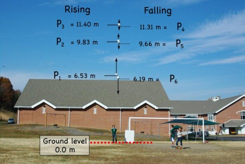
If you throw a soccer ball up into the air and take a quick series of photographs you can capture the motion of the ball over time. The height of the ball can be measured off the photographs, which can then be used for some interesting physics and mathematics analysis. This assignment focuses on the analysis. It starts with the height of the ball and the time between each photograph already measured (Figure 1 and Table 1).

projectile-diagram-plain — Figure 1. Height of a thrown ball, measured off a series of photographs. The photographs have been overlaid to create this image of multiple balls.

Table 1: Height of a thrown soccer ball over a period of approximately 2.5 seconds. This data were taken from a previous experiment on projectile motion.

Photo	Time (s)	Measured Height (m)
P₀	0	1.25
P₁	0.436396062	6.526305882
P₂	0.849230104	9.825317647
P₃	1.262064145	11.40310588
P₄	1.674898187	11.30748235
P₅	2.087732229	9.657976471
P₆	2.50056627	6.191623529

Assignment

Pre-Algebra: Draw a graph showing the height of the ball (y-axis) versus time (x-axis).
Algebra/Pre-calculus: Determine the equation that describes the height of the ball over time: h(t). Plot it on a graph.
Calculus: Determine the equation that shows how the velocity of the ball changes over time: v(t).
Calculus: Determine the equation that shows how the acceleration of the ball changes with time: a(t)
Physics: What does this all mean?

Flying Robotics

A fascinating demonstration of using modeling to maneuver flying robots (quadrocopters).

Rates of change: 4 cm/liter

Apollo_11_first_stage_separation — The first stage rocket booster separates. Image from NASA via Wikipedia.

Fully loaded, the first stage of the Saturn V rockets that launched the Apollo missions would burn through a liter of fuel for every four centimeters it moved. That’s 5 inches/gallon, which, for comparison, is a lot less than your modern automobile that typically gets over 20 miles/gallon.