C.G.P.Grey lays out the problems with the U.S.A’s current “first past the post/winner take all” voting system and then explains how to fix them:
The problems:
Minority rule: You can win with less than half the vote (at least in the beginning).
Inevitable, unavoidable, two-party system evolves over time.
Third-parties become spoilers; the better a third-party does the worse it is for their voters because it takes away votes from the other party they would favor.
Pepper plant responding to being watered. These images were taken over the course of two hours.
During class on Friday, I watered my Chinese five-color hot pepper plant for the first time in three days. It responded quite well, helping to illustrate one reason (to maintain their rigidity/prevent wilting) why plants need water. I did this because I was curious about how fast plants respond to water, and with the data from the images I should be able to demonstrate what a scientific report should look like.
The full plant’s response:
Notes
The original camera images were cropped for the gif-animation using Imagemagick’s convert
convert $i -crop 500x400+1550+1100 crop-$i
The image file sequences were converted to mp4 video using ffmpeg (instructions here):
Dan Ariely concludes (video by RSA) that making people think about morality increases the likelihood that they’ll act honestly.
People try to balance the benefiting they gain from cheating against being able to feel good about themselves by being honest. While very few people tend to cheat a lot, many people cheat a little and self-rationalize their dishonesty.
Our school has adopted a short honor code that we’ll ask students to write at the top of tests and other assignments that is intended to remind them of their moral obligations.
Based on one of Ariely’s other conclusions, I’m also considering having students confess their in-class transgressions — talking out of turn; improper use of technology — every month or so, since this type of thing also seems to encourage probity.
The video shows 300 seconds of purely exponential growth (uninhibited), captured from the exponential growth VAMP scenario. Like the exponential growth function itself, the video starts off slowly then gets a lot more exciting (for a given value of exciting).
The modeled growth is based on the exponential growth function:
(1)
where:
N = number of cells (or concentration of biomass);
N0 = the starting number of cells;
r = the rate constant, which determines how fast growth occurs; and
t = time.
Finding the Rate Constant/Doubling Time (r)
You can enter either the rate constant (r) or the doubling time of the particular organism into the model. Determining the doubling time from the exponential growth equation is a nice exercise for pre-calculus students.
Let’s call the doubling time, td. When the organism doubles from it’s initial concentration the growth equation becomes:
divide through by N0:
take the natural logs of both sides:
bring the exponent down (that’s one of the rules of logarithms);
remember that ln(e) = 1:
and solve for the doubling time:
Decay
A nice follow up would be to solve for the half life given the exponential decay function, which differs from the exponential growth function only by the negative in the exponent:
A useful calculus assignment would be to determine the growth rate at any point in time, because that’s what the model actually uses to calculate the growth in cells from timestep to timestep.
The growth rate would be the change in the number of cells with time:
starting with the exponential growth equation:
since we have a natural exponent term, we’ll use the rule for differentiating natural exponents:
So to make this work we’ll have to define:
which can be differentiated to give:
and since N0 is a constant:
substituting in for u and du/dt gives:
rearranging (to make it look prettier (and clearer)):
(2)
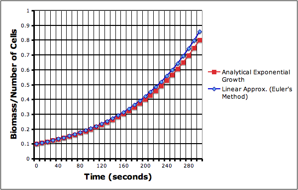
Numerical Methods: Euler’s method
With this formula, the model could use linear approximations — like in Euler’s method — to simulate the growth of the biomass.
First we can discretize the differential so that the change in N and the change in time (t$) take on discrete values:
Now the change in N is the difference between the current value Nt and the new value Nt+1:
Now using this in our differentiated equation (Eq. 2) gives:
Which we can solve for the new biomass (N^t+1):
to get:
This linear approximation, however, does introduce some error. The approximated exponential growth curve (blue line) deviates from the analytical equation. The deviation compounds itself, getting worse exponentially, as time goes on.
This is the first, basic but useful product of my summer work on the IMPS website, which is centered on the VAMP biochemical model. The VAMP model is, as of this moment, still in it’s alpha stage of development — it’s not terribly user-friendly and is fairly limited in scope — but is improving rapidly.
A billion, in continental Europe is, a million squared ( 1,000,0002 = 1,000,000,000,000), but in the English speaking world, a billion is only a thousand million (1,000,000,000). numberphile goes into the beautiful, mathematical logic of the longer form (i.e. the continental system).
Of course, the “simplest” system, which avoids all the potential for miscommunication, is the standard scientific notation, where 1,000,000,000 is written as 1×10⁹ (or just 109).