The reintroduction of wolves to Yellowstone National Park resulted in enormous changes to the ecology: more plants and animals as the wolves reduced the deer population and changed the deers’ behavior. The change in vegetation resulted in stabilization of the rivers, so the wolves changed the geomorphology of the park as well.
Headless Pi Zero
Pi Zero‘s are even cheaper versions of the Raspberry Pi. The price you pay is that they’re harder to connect to since all the ports are small (micro-USB’s and mini-HDMI’s), so you need adapters to connect to keyboards, mice, and monitors. However, if you have the wireless version (Pi Zero W) you can set it up to automatically connect to the WiFi network, and work on it through there using the command line. This is a brief summary of how to do this (it’s called a “headless” setup) based on Taron Foxworth’s instructions. It should work for the full Raspberry Pi as well.
Set up the Operating System
You can install the Raspbian Stretch (or Raspbian Lite which does not include the desktop GUI that you will not use) on a SD card (I used 8 or 16 Gb cards).
- Download Raspbian.
- SD Card Formatter to format the SD Card. It’s pretty quick, just follow the instructions.
- Etcher: to install the operating system on the SD Card
Set up automatic connection to WiFi
You may have to remove and reinsert the SD Card to get it to show up on the file system, but once you have you can set it up to automatically connect to WiFi by:
- Go into the
/bootpartition (it usually shows up as the base of the SD Card on your file manager) and create a file named “ssh”. - Create a text file called “wpa_supplicant.conf” in the /boot folder, and put the following into it, assuming that the wifi router you’re connecting to is called “myWifi” and the password is “myPassword”.
country=US
ctrl_interface=DIR=/var/run/wpa_supplicant GROUP=netdev
update_config=1

network={
 ssid="myWifi"
 scan_ssid=1
 psk="myPassword"
 key_mgmt=WPA-PSK
}
Now put the SD Card into the Pi and plug in the power.
Find the IP address
First you have to find the Pi on the local network. On Windows I use Cygwin to get something that looks and acts a bit like a unix terminal (on Mac you can use Terminal, or any shell window on Linux).
To find the ip address of your local network use:
on Windows:
> ipconfig
look for the “IPv4 Address”.
Mac (and Linux?)
> ifconfig
look under “en1:”
Connecting
To connect you use ssh on the command line (Mac or Linux) or something like Putty
Static IP
Without a static IP address it is possible that the Pi’s IP address will change occasionally. I followed the instructions on Circuit Basics and MODMYPI, but basically you have to:
- Identify your network information:
- Find your Gateway:
> route -ne
> cat /etc/resolv.conf
interface wlan0
static ip_address=10.0.0.99
static routers=10.0.0.1
static domain_name_servers=75.75.75.75
A Web Server
Adding a webserver (apache with php) is pretty easy as well, just run the commands (from the Raspberry Pi Foundation)
Apache web server:
sudo apt-get install apache2 -y
PHP for server-side scripting
sudo apt-get install php libapache2-mod-php -y
Now your can find the webpage by going to the ip address (e.g. http://10.0.0.1).
The actual file that you’re seeing is located on the Pi at:
/var/www/html/index.html
You will probably need to change the ownership of the file in order to edit it by running:
> sudo chown pi: index.html
Looking Behind the Statistics
For my statistics students, as we approach the end of the course, to think about the power of statistics and how using them, even with the best intentions, can go wrong.
https://www.npr.org/podcasts/510298/ted-radio-hour: Go to JANUARY 26, 2018. Can We Trust The Numbers?
The Wall (Mural)
Our seniors wanted to leave a mark, so after their initial application to paint the outside wall of the gym was turned down, they went with a mural on the inside–in our Makerspace.
For this project, we wanted to create a mural on the basementnasium wall. First, we measured the wall and went to Home Depot to get enough paint, paint brushes, drop cloths, and tape. Then, after cleaning the wall with a damp cloth, we covered the wall with tape in a triangular pattern similar to one we found online. After that, we used pencil to mark each triangle with a letter corresponding to one of the six colors that we bought. It took us the majority of the project to paint 3-4 coats on each triangle, and on the last day we pulled it the tape and touched up any mistakes with white paint.
Throughout this project, we found out that some people know how to paint, some people learned, and others didn’t learn. BUT IT WAS SO MUCH FUN!
-Team: Elliott, Abby, John, Zoe, Mary, Annemarie, and Josiah
-Abby R.
Longboard
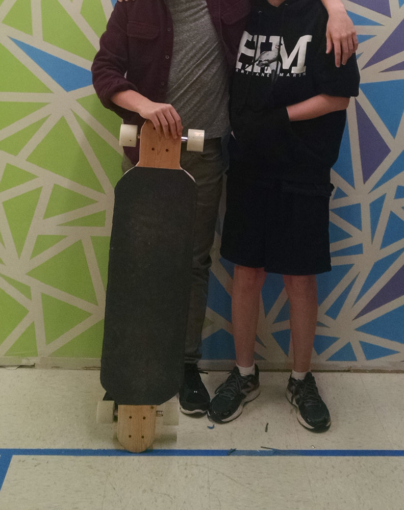
Finishing came afterwards.
For my makerspace project I made a longboard. What went well with the board was the wheels and trucks, it was a simple hole in the wood and screwing the trucks almost no measuring on my part. What didn’t go so well was the measuring and cutting of the board, it took me a full day to get all the measurements exact and even then they didn’t come out so good. What I would do next time is get a cnc machine so it does the measuring and gets the cuts exact every time. We could mass produce longboards with ease. If i did it again without a cnc machine i would get the measurements beforehand and then it would make measuring a lot easier.
– Isaac L.
Making Stools

After building our vegetable boxes, I had one of the students use some of the wood scraps to make some small stools. They make it easier for us to sit cross-legged on the floor. This last interim, as a small side project, another student chose to upholster them:
During the interim, I worked on upholstering small wooden stools that Dr. Urbano had made. I worked in the basmentnasium and only used the materials available there. I used thin layers of foam from an old couch to pad the wooden seat; if the foam was too thin then I used two layers. I covered the foam and the seats’ edges with fabric Dr. Urbano brought: a burlap rice bag and old curtains. I attached the fabric to the bottom of the wooden seat with a staple gun; I attached it tight enough to keep the foam in place.
– Mary R.
Preparing Students for a Technological Future
I’m currently preparing a proposal to create a laboratory of digital fabrication machines–a CNC, a laser, and a vinyl cutter–and one of the questions I’m answering is about how the proposed project would prepare students for a technology-rich future. What you see below is my first response to this prompt. It’s a bit longer than I have space for in the proposal, and probably a bit too philosophical, but before I cut it down I wanted to post this draft because it does a reasonable job of encapsulating my philosophy when it comes to teaching technology:
Preparation for a technology rich future is less about preparing for specific technologies and more about getting students to have a growth mindset with respect to technology. We are living in a truly wonderful moment in history. Technological tools are rapidly expanding what we as individuals can accomplish. They are allowing us to see farther (think about remote sensing like lidar and tomography), collate more information (especially with more and more data becoming publicly available), and create things that push the limits of our imaginations. Indeed, to paraphrase a former student, we are already living in the future.
To prepare students to live and thrive in this ever-evolving present we need to demystify technology and give students the intellectual tools to deal with the rapid change. We can start by letting them peek into the black boxes that our technological devices are rapidly becoming.
We request electronics stations and tool kits not just to build things, but to be able to take them apart and look inside. Students greatly enjoy dissassembling and reassambling computers, for example, which provides younger students a good conceptual understanding of how most modern devices work. This foundation helps when they start building circuits of their own and realize what they really want to do is to control them–making lights blink and turning motors for example–and this is when they will start working with Raspberry Pi computers, Arduino microcontrollers and programming.
As students start to build (and even before really), they naturally start thinking about design. We all have an affinity for the aesthetic. If you’ve ever had the opportunity to see a laser in action, you’ll remember your sense of fascination the first time you saw someone’s design emerging from the raw material right before your eyes. Thus we get into graphic design, computer aided design (CAD) and computer aided manufacturing (CAM) and the digital fabrication machines we propose.
By the time they’re done with this curriculum, we intend that students will have developed an intimate familiarity with the technological world–including the ability to create and design their own, which prepares them for the technological future.
Vegetable Boxes
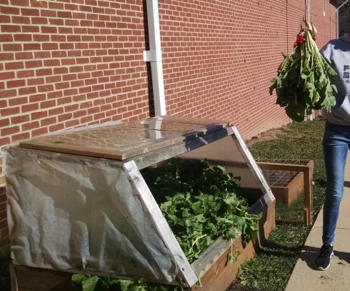
Two years ago we bought a greenhouse. It was aluminum framed with plastic panels. Unfortunately, its profile was not as wind-resistant as it needed to be for our campus. So last semester we built three vegetable boxes and salvaged the plastic panels from the greenhouse to build low-profile cold frames. These turned out quite nicely, and the Middle School’s Student-Run-Business’ Gardening Department have been experimenting with different types of produce.

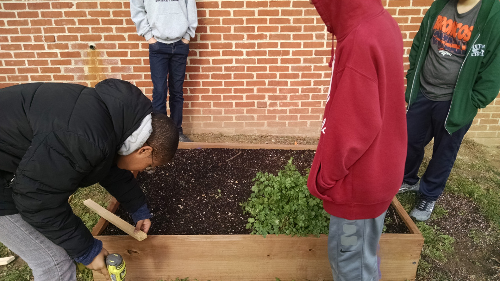
The wood for the raised beds and the frames for the cold frames were purchased using funds from a grant by the Whole Kids Foundation and the pieces cut at the TechShop.