Energy and matter can’t just disappear. Energy can change from one form to another. As a thrown ball moves upwards, its kinetic energy of motion is converted to potential energy due to gravity. So we can better understand systems by studying how energy (and matter) are conserved.
Energy Balance for the Earth
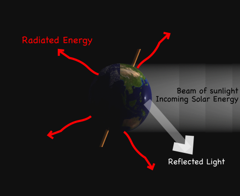
Let’s start by considering the Earth as a simple system, a sphere that takes energy in from the Sun and radiates energy off into space.
Incoming Energy
At the Earth’s distance from the Sun, the incoming radiation, called insolation, is 1367 W/m2. The total energy (wattage) that hits the Earth (Ein) is the insolation (I) times the area the solar radiation hits, which is the area a cross section of the Earth (Acx).

Given the Earth’s radius (rE) and the area of a circle, this becomes:

Outgoing Energy
The energy radiated from the Earth is can be calculated if we assume that the Earth is a perfect black body–a perfect absorber and radiatior of Energy (we’ve already been making this assumption with the incoming energy calculation). In this case the energy radiated from the planet (Eout) is proportional to the fourth power of the temperature (T) and the surface area that is radiated, which in this case is the total surface area of the Earth (Asurface):

The proportionality constant (σ) is: σ = 5.67 x 10⁻⁸ W m-2 K-4
Note that since σ has units of Kelvin then your temperature needs to be in Kelvin as well.
Putting in the area of a sphere we get:

Balancing Energy
Now, if the energy in balances with the energy out we are at equilibrium. So we put the equations together:


cancelling terms on both sides of the equation gives:

and solving for the temperature produces:

Plugging in the numbers gives an equilibrium temperature for the Earth as:
T = 278.6 K
Since the freezing point of water is 273K, this temperature is a bit cold (and we haven’t even considered the fact that the Earth reflects about 30% of the incoming solar radiation back into space). But that’s the topic of another post.


 ,
, ,
,


.svg)