I tend to let my students have a lot of freedom to use their myriad technological devices as they will. Just as long as they use them responsibly (i.e. for academics during class time). What’s most interesting these days is seeing how they combine the various electronics.
Working with pen, paper, tablet and laptop.
This Chemistry student is referring to her textbook on the iPad, while she creates a presentation on her laptop. Yet pen and paper are still integral parts of the process.
Given the idea that “learning situated in meaningful contexts is often deeper and richer than learning in abstract contexts,” (Lillard, 2007), I’ve been trying to orient our robotics program toward developing devices that we can use at school. Not only can these devices serve a useful purpose, but their presence around the school can, perhaps, inspire other students to want to make their own.
To this end, one of our first practical projects is a timer (by Joe A.) for when students give their presentations in Chemistry class. For the last round of presentations they had 20 minutes, so I had Joe build the circuits and program the Arduino to make the green light to be on for 15 min, the yellow on for 4 min, the red for 1 min, and then the piezoelectric buzzer would go off for 5 seconds and the red light would start blinking.
Joe did an awesome job, and the timer worked remarkably well. I did what we wanted it to do, and it actually worked to help them keep their presentations under time.
Students explore the massive, spheroidally weathered boulders at Elephant Rocks State Park.
We stopped at the Elephant Rocks State Park our way down to Eminence MO for our middle school immersion trip. The rocks are the remnants of a granitic pluton (a big blob of molten rock) that cooled underground about 1.5 billion years ago. As the strata above the cooled rock were eroded away the pressure release created vertical and horizontal cracks (joints). Water seeped into those joints, weathered the minerals (dissolution and hydrolysis mainly), and eroded the sediments produced, to create the rounded shapes the students had a hard time leaving behind.
This was a great stop, that I think we’ll need to keep on the agenda for the next the next trip. I did consider stopping at the Johnson’s Shut-Ins Park as well, but we were late enough getting to Eminence as it was. Perhaps next time.
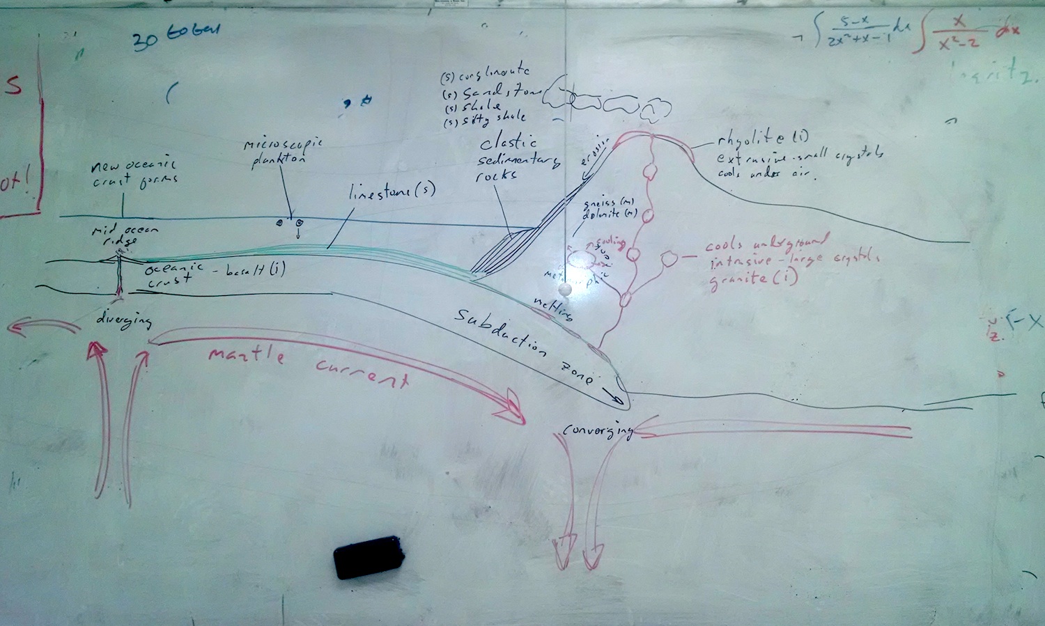
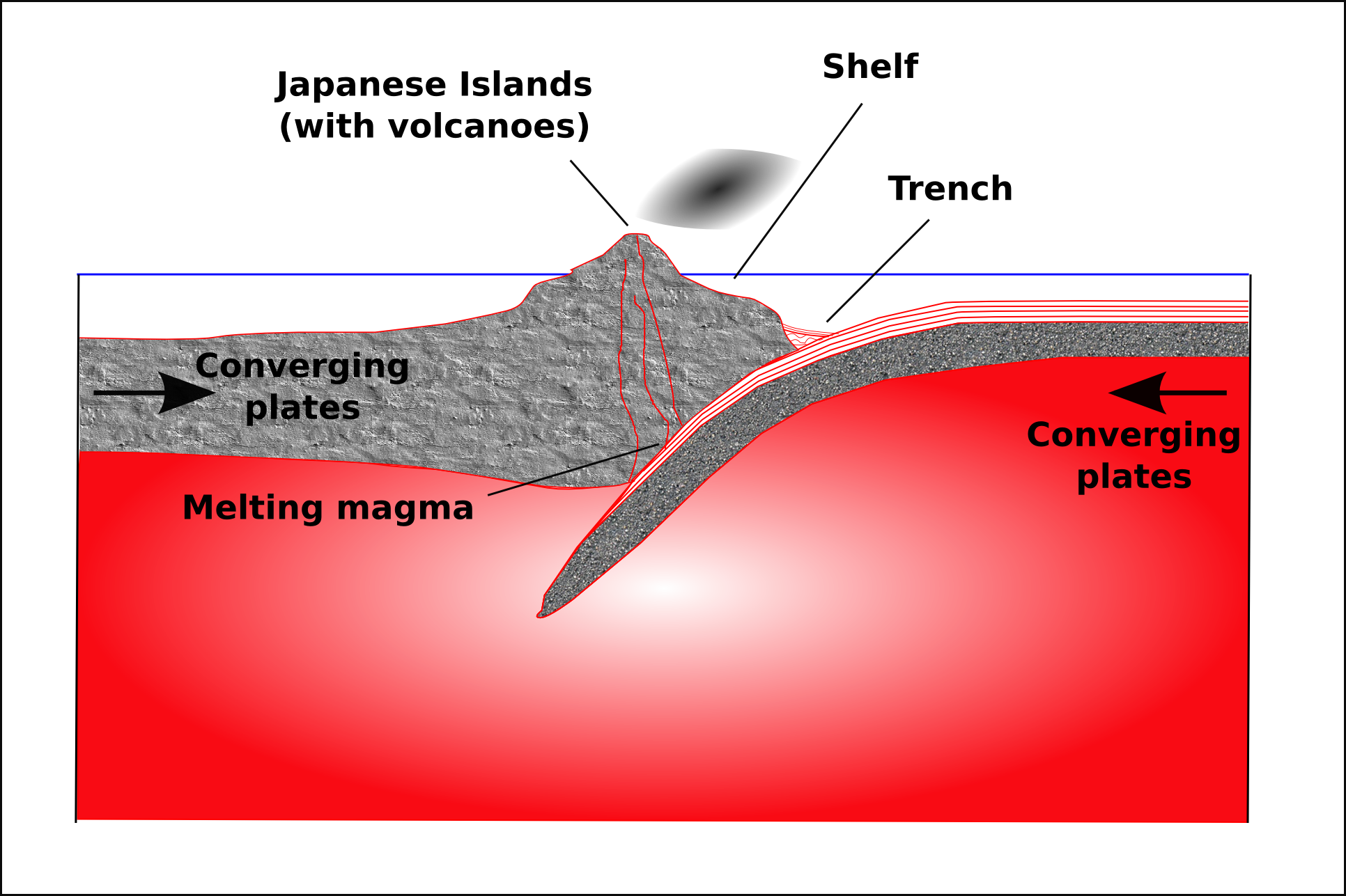
The picture of a convergent tectonic boundary pulls together our immersion trip to Eminence, and the geology we’ve been studying this quarter. We saw granite boulders at Elephant Rocks; climbed on a rhyolite outcrop near the Current River; spelunked through limestone/dolomitic caverns; and looked at sandstone and shale outcrops on the road to and from school.
The subducting plate melts producing volatile magma.
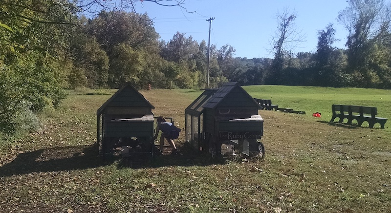
Last year, our middle schoolers named their business Chicken Middle. I was a bit skeptical, but the name stuck. This year, thanks to a lot of help from the school community (thanks to the R’s for the Ruby Coops), we finally have chickens (thanks to Mrs. C. for fostering chicks for us over the summer).
And today, we had our first egg. The students were a little excited.
It looks a little lonely sitting there by itself in the egg carton (thanks to Mrs. D., Mrs. P., and everyone else who donated egg cartons), but with a little luck it will have lots of company soon.
The Tabletop Whale blog by Elanor Lutz, has a focus on scientific illustration. It is a wonderful intersection of science, math and art, such as in this beautiful animation of a muscle in motion.
Perhaps not surprisingly, my middle school students have a difficult time wrapping their heads around the idea of multiple frames of reference. We were in a canoe on the Current River and I asked the student paddling in the rear of the boat to look at me and answer the question, “Are we in the canoe moving, or are we steady in one spot and everything around us moving?”
This resulted in some serious cognitive processing. And she still has not gotten back to me with an answer.
Another student, faced with the same question, thought it over overnight and concluded that it was a riddle. He figured the correct answer was that the canoe was moving and the land was still. I asked him to think about it a little more (because he was only half right).
Interestingly enough, I’ll be teaching my Advanced Physics class this block, and the first chapter has a neat little section on coordinate systems. I’m curious to see if the 11th and 12th graders have an easier time with the concept.