This little embeddable, interactive app uses nth order polynomials to approximate a few curves to demonstrate the Taylor Series.
Tag: graphing
Practicing Plotting Points on the Co-ordinate Plain
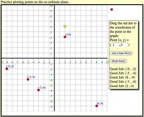
Pre-Algebra class starts next week, so in preparation for one of the early lessons on how to plot x,y co-ordinates, I put together an interactive plotter that lets students drag points onto the co-ordinate plain.
Usage
The program generates random coordinate pairs within the area of the chart (or you can enter values of the coordinates yourself):
- Clicking the “Show Point” button will place a yellow dot at the point.
- When you’re confident you understand how the coordinate pairs work, you can practice by dragging the red dot to where you think the point is and the program will tell you if you’re right or not.
About the Program
This interactive application uses the jQuery and KineticJS javascript libraries. The latter library in particular is useful for making the HTML5 canvases interactive, so you can click on points on the graph and drag them.
When I have some time, after classes settle down, I’ll see if I can figure out how to embed this type of app into this (WordPress) blog. KineticJS is based off HTML5 canvases, which is what I use for the other interactive graphs I’ve posted, so it shouldn’t be terribly hard (at least in principle).
Solving Quadratic Equations
So here we have a little grapher that solves quadratic equations visually. Just enter the coefficients in the equation.
[inline]
Quadratic Equation: y = a x2 + b x + c
Enter:
y =
x2 +
x +
Solution:
Analytical solution by factoring (with a little help from the quadratic equation if necessary).
[script type=”text/javascript”]
var width=500;
var height=500;
var xrange=10;
var yrange=10;
mx = width/(2.0*xrange);
bx = width/2.0;
my = -height/(2.0*yrange);
by = height/2.0;
function draw_9114(ctx, polys) {
t_9114=t_9114+dt_9114;
//ctx.fillText (“t=”+t, xp(5), yp(5));
ctx.clearRect(0,0,width,height);
polys[0].drawAxes(ctx);
ctx.lineWidth=2;
polys[0].draw(ctx);
polys[0].write_eqn(ctx);
//polys[0].y_intercepts(ctx);
polys[0].x_intercepts(ctx);
//write intercepts on graph
ctx.fillText (‘x intercepts: (when y=0)’, xp(9), yp(8));
if (polys[0].x_intcpts.length > 0) {
line = “0 = “;
for (var i=0; i
line = line + “(x “+sign+” “+ Math.abs(polys[0].x_intcpts[i].toPrecision(2))+ “)”;
}
ctx.fillText (line, xp(9), yp(7));
// if (polys[0].order == 2 ) {
// if (polys[0].x_intcpts[0] > 0.0) { sign1=”-“;} else {sign1=”+”;}
// if (polys[0].x_intcpts[1] > 0.0) { sign2=”-“;} else {sign2=”+”;}
// ctx.fillText (‘0 = (x ‘+sign1+” “+Math.abs(polys[0].x_intcpts[0])+”) (x “+sign2+Math.abs(polys[0].x_intcpts[1])+”)”, xp(9), yp(7));
// }
for (var i=0; i
“;
solution = solution + ‘Factoring: ‘;
if (polys[0].x_intcpts.length > 0) {
solution = solution + ‘0 = ‘;
for (var i=0; i
solution = solution + “(x “+sign+” “+ Math.abs(polys[0].x_intcpts[i].toPrecision(2))+ “)”;
}
solution = solution + ‘
‘;
solution = solution + ‘Set each factor equal to zero:
‘;
for (var i=0; i
solution = solution + “x “+sign+” “+ Math.abs(polys[0].x_intcpts[i].toPrecision(2))+ ” = 0 “;
}
solution = solution + ‘
and solve for x:
‘;
for (var i=0; i
}
document.getElementById(‘equation_9114’).innerHTML = solution;
}
else if (polys[0].order == 1) {
solution = solution + ‘
‘;
solution = solution + “y = “+” “+Math.abs(polys[0].b.toPrecision(2))+” x “+ polys[0].csign+” “+Math.abs(polys[0].c.toPrecision(2))+”
“;
solution = solution + ‘
Set y=0 and solve for x:
‘;
solution = solution + ” 0 = “+” “+Math.abs(polys[0].b.toPrecision(2))+” x “+ polys[0].csign+” “+Math.abs(polys[0].c.toPrecision(2))+”
“;
solution = solution + ‘ ‘;
solution = solution + (-1.0*polys[0].c).toPrecision(2) +” = “+” “+Math.abs(polys[0].b.toPrecision(2))+” x “+”
“;
solution = solution + ‘ ‘;
solution = solution + (-1.0*polys[0].c).toPrecision(2)+”/”+polys[0].b.toPrecision(2)+” = “+” x “+”
“;
solution = solution + ‘ ‘;
solution = solution + “x = “+ (-1.0*polys[0].c/polys[0].b).toPrecision(4)+”
“;
document.getElementById(‘equation_9114’).innerHTML = solution;
}
}
//init_mouse();
var c_9114=document.getElementById(“myCanvas_9114”);
var ctx_9114=c_9114.getContext(“2d”);
var change = 0.0001;
function create_lines_9114 () {
//draw line
//document.write(“hello world! “);
var polys = [];
polys.push(addPoly(1,6, 5));
// polys.push(addPoly(0.25, 1, 0));
// polys[1].color = ‘#8C8’;
return polys;
}
var polys_9114 = create_lines_9114();
var x1=xp(-10);
var y1=yp(1);
var x2=xp(10);
var y2=yp(1);
var dc_9114=0.05;
var t_9114 = 0;
var dt_9114 = 100;
//end_ct = 0;
var st_pt_x_9114 = 2;
var st_pt_y_9114 = 1;
var move_dir_9114 = 1.0; // 1 for up
var a_coeff_9114 = document.getElementById(“a_coeff_9114″);
a_coeff_9114.value = polys_9114[0].a+””;
var b_coeff_9114 = document.getElementById(“b_coeff_9114″);
b_coeff_9114.value = polys_9114[0].b+””;
var c_coeff_9114 = document.getElementById(“c_coeff_9114″);
c_coeff_9114.value = polys_9114[0].c+””;
//document.write(“test= “+c_coeff_9114.value+” “+polys_9114[0].c);
//setInterval(“draw_9114(ctx_9114, polys_9114)”, dt_9114);
draw_9114(ctx_9114, polys_9114);
a_coeff_9114.onchange = function() {
polys_9114[0].set_a(parseFloat(this.value));
draw_9114(ctx_9114, polys_9114);
}
b_coeff_9114.onchange = function() {
polys_9114[0].set_b(parseFloat(this.value));
draw_9114(ctx_9114, polys_9114);
}
c_coeff_9114.onchange = function() {
polys_9114[0].set_c(parseFloat(this.value));
draw_9114(ctx_9114, polys_9114);
}
[/script]
[/inline]
Hopefully, this can help students learn about factoring and quadratics in a more graphical way.
Notes:
This is my first interactive post. I use Javascript in combination with HTML5. Now I need to figure out how to interact with the image itself, instead of the textboxes.
Straight Lines
[inline]
[script type=”text/javascript”]
var width=500;
var height=500;
var xrange=10;
var yrange=10;
mx = width/(2.0*xrange);
bx = width/2.0;
my = -height/(2.0*yrange);
by = height/2.0;
function draw8587(ctx, polys) {
t=t+dt;
//ctx.fillText (“t=”+t, xp(5), yp(5));
ctx.clearRect(0,0,width,height);
polys[0].drawAxes(ctx);
//drawAxes(ctx);
ctx.lineWidth=3;
//ctx.beginPath();
//ctx.moveTo(x1,y1);
//ctx.lineTo(x2,y2);
//ctx.stroke();
//ctx.closePath();
//y2+=dyp(dy);
// add polynomial timing
// First move (from y=0 to y=1)
if (polys[0].c < 1.0) {
polys[0].c = polys[0].c + 2.0*dt*change*move_dir;
}
// Second move (change from y=1 to y=0.5x+1)
else if (polys[0].b < 0.5) {
polys[0].b = polys[0].b + dt*change*move_dir;
polys[0].order = 1;
}
// Third move (change from y=0.5x+1 to y=0.5x+4)
else if (polys[0].c < 4.0) {
polys[0].c = polys[0].c + 2.*dt*change*move_dir;
//polys[0].order = 1;
}
else {
//move_dir = move_dir * -1;
end_ct = end_ct + dt;
if (end_ct >= dt*40) {
polys[0].a = 0;
polys[0].b = 0;
polys[0].c = 0;
polys[0].order = 0;
}
}
ctx.textAlign=”center”;
ctx.textBaseline=”alphabetic”;
ctx.font = “14pt Arial”;
ctx.fillStyle = ‘#f00’;
ctx.fillText (“Equation of a Line”, xp(-5), yp(9));
ctx.fillText (“y = mx + b”, xp(-5), yp(5));
ctx.font = “12pt Arial”;
//ctx.fillText (“y = “+polys[0].b.toPrecision(1)+”x + “+ polys[0].c.toPrecision(2), xp(-5), yp(7));
ctx.fillText (“b = intercept = “+polys[0].c.toPrecision(2), xp(-7), yp(3));
//draw polynomials Here’s a prototype for showing how the equation of a straight line changes as you change its slope (m) and intercept (b): It starts with an horizontal line along the x-axis, where the slope is zero and the intercept is zero: The line moves upward, but stays horizontal, until the intercept is 1.0: The slope increases from horizontal (m = 0), gradually, until the slope is 0.5: Finally, we move the line upwards again, without changing the slope (m = 0.5), until the intercept is equal to 4.0: Now I just need to figure out how to make them interactive.
ctx.lineWidth=3;
for (var i=0; i
![]()
![]()
![]()
![]()
![]()
Malthusian Growth
I think I may fairly make two postulata.
First, That food is necessary to the existence of man.
Secondly, That the passion between the sexes is necessary and will remain nearly in its present state.
— Malthus (1798): An Essay on the Principle of Population via The Concise Encyclopedia of Economics
“Malthusian” is often used as a derogatory term to refer to alarmist predictions that we’re going to run out of some natural resource. I’m afraid I’ve used the term this way myself, however, according to Lauren Landsburg at the Concise Encyclopedia of Economics, Malthus is being unfairly maligned. He wasn’t actually predicting catastrophe but wondering why the catastrophes don’t usually happen.
What Thomas Malthus did, in 1798, was point out that while populations grow at a geometric rate – the U.S. population, he noticed, doubled every 25 years – but resources, like food, only increase at an arithmetic rate. As a result, any naturally growing population will eventually run out of resources.
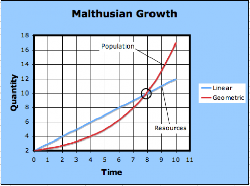
The linear equation has the form:
![]()
where y is the quantity produced, t is time (the independent variable), and m and b are constants. This should not look to unfamiliar to students who’ve had algebra.
The geometric equation is a little more complicated:
![]()
here a, g and c are constants. g is the most important, because it’s the growth rate – the higher g is the faster the curve will rise. You can play around with the coefficients and graph in this Excel spreadsheet .
At any rate, after the curves intersect, the needs of the population exceeds how much it can produce; this is the point of Malthusian catastrophe.
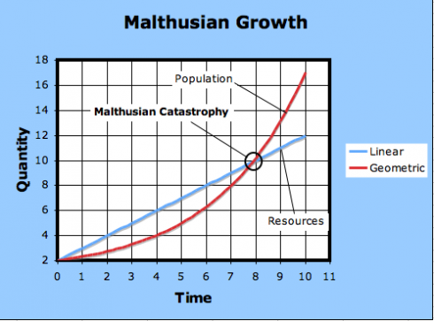
The observation is, indeed, so stark that it is still easy to lose sight of Malthus’s actual conclusion: that because humans have not all starved, economic choices must be at work, and it is the job of an economist to study those choices.
— Landsburg (2008): Thomas Robert Malthus from The Concise Encyclopedia of Economics.
What’s Needed for a Nation’s Peace
The Fund for Peace has been doing a lot of thinking about what it takes for a country to be considered peaceful, and what it takes for a state to fail. For the last seven years they’ve been putting together maps of the world with an index of how stable different countries are.
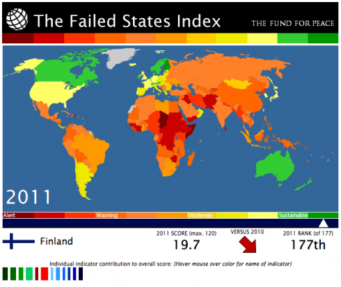
While it’s pretty in-depth and makes for rather sobering reading, it’s worth taking a look at the criteria they’ve come up with to determine a country’s stability. It may be useful to include some of this information in the cycle where we focus on peace.
Their criteria for instability include:
- Demographic pressure (such as having too many young adults, as we’ve seen in Egypt)
- Amount of refugees and internally displaced peoples (refugees are people who’ve crossed international borders). Both leaving or entering refugees can undermine stability.
- Historical Injustice – communities can have an understandably hard time forgetting the past, just look at Isreal/Palestine.
- Brain Drain – when countries start to fail, the first to leave are the ones who can afford to. Yet these intellectuals and professionals, with their college degree are vital for creating a stable and prosperous country.
- Inequality – especially when driven by active discrimination (wealth inequality is something to watch out for).
- Economic decline – pushes trade into the black market and increases criminality and corruption.
- Illegitimacy of the state – if people don’t believe the people in government have everyone in the country’s best interests at heart, and are only looking out for themselves and their friends, then there’s probably going to be trouble.
- Public Services go kaput – It’s a really bad sign when the government can meet people’s basic needs – like picking up the garbage.
- The Rule of Law goes kaput – when you’re ruled by the caprice of men, and your rights under the law are not respected, you may begin to consider and agitate for other options for government.
- Personal Armies – forces that are tied to individual leaders, like private militias or super-secret police for example, are very damaging to a country’s cohesion.
- Fighting elites – healthy countries need robust arguments in their political class – think checks and balances – but it can go too far and lead to things like extreme nationalism and ethnic cleansing.
- Invasion – both overt invasion and covert meddling in the affairs of a country are unhealthy for that state’s stability.
It’s also very nice that you can download their index data as a MS Excel spreadsheet, which you can let students analyze to answer their own research questions. For example, I was wondering what was the difference between the best, the worst and the USA, so I plotted this graph.
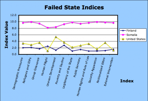
The USA is much closer to Finland than Somalia, thank goodness, but should probably watch out for that Uneven Development (wealth inequality).
I think something like this would make a good experiential exercise for the science of geography.