Differentiation Using Limits

We can use the idea of limits to come up with some general relationships between functions and their slopes. Take, for example, the last project where we found the slope of the function y = x2 at the point where x = 3:
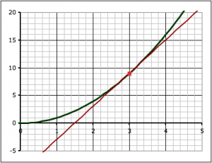
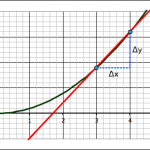
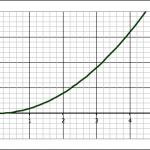
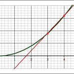
The green line is the curve y = x2 and the straight red line is the tangent to the curve at the point where x = 3 (i.e. at (3,9)).
Finding the approximate slope using a forward difference.

We found the slope of the tangent line at the point (3,9) by a series of approximations. First we took two points on the curve, (3,9) and (4,16) and found the slope between those two points.

The equation for slope can be written in any of these three ways:

slope-line

we find the exact slope by taking points on the line closer and closer together (which means that Δx is getting smaller and smaller). In math-speak, we’re saying that we’re taking the limit of the slope equation as Δx approaches zero.

slope-limit

Since we’re taking Δx to zero we might as well ask what happens to the slope when Δx is equal to zero.

slope-undef

As we can see from the equation, we end up with zero on the denominator, which makes the whole thing undefined, which we really do not want.

But what if we can rearrange things to get the Δx out of the denominator?

Let’s rewrite the equation y = x2 as a function:

 f(x) = x^2

So the point we’re interested in find the slope at is just (x, f(x)), which in this case happens to be (3, 9), but we’re not going to be using the actual numbers anymore so we can come up with a more general relationship.

To find the slope we find the point where the value on the x-axis is x and the value on the y-axis is f(x).

Now, and this is often the tricky part, the second point we use is going to have an x value of x + Δx:

For the second point, the x value we use is the first x offset by Δx.

which means that the value on the curve is f(x+Δx):

Our second point is where the x value is x+Δx and the y value is f(x+Δx).

So lets carefully observe the notation here. To find the slope of a line we can use the equation:

slope-basic
But with the function notation:

  • y1 = f(x)
  • y2 = f(x+Δx)

so:

slope-f

Now watch very carefully as I replace the function notation with the actual functions, specifically:

  • f(x) = x2
  • f(x+Δx) = (x+Δx)2

to give:

slope-f2

and if you understand how this, we’re almost all there, because the rest is algebra.

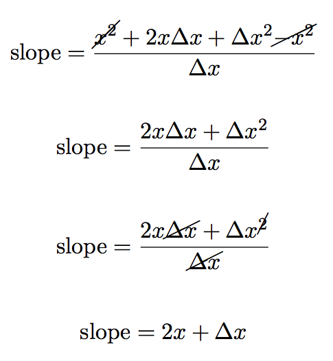
We simplify the equation above by expanding the numerator.

slope-f3

now we can subtract the similar terms (x2) and divide through by Δx to get:

slope-f4

But remember we don’t just want the slope, we want to find the slope where Δx approaches zero:

slope-lim2

The problem before was that if we made Δx = 0 the equation would be undefined. But now, however, as Δx = 0 the second term in the equation just goes to zero:

slope-f5

leaving us just with the first term 2x:

slope-diff

Remember that we were trying to do this at the point where x = 3. So if we put x = 3 into this equation we get:

slope-diff2

Which we know is the right answer because we did the very problem by hand already.

but now however we’ve come up with a more general equation for the slope. With it we can easily find the slope of our curve at any point along the curve!

For example, what is the slope of the curve when x = 0:

slope-diff4

Notation

Now it’s a bit cumbersome to write the limit as Δx goes to zero every time, so we’ll instead call our equation for the slope of the line the differential, and we’ll give it the notation as the function prime:

i.e. if we have a function f(x) = x2:

diff_notation-1

we write its differential as:

diff-notation-2

To confuse things (at least for the moment) there are a number of ways of writing the differential (the different methods are useful in different contexts), so you will see things like:

diff-notation-3

So now that we know how to find the differential using limits, we’ll practice finding the differential of polynomial functions and see if we can find a general pattern that allows us to bypass the whole limits thing altogether.

Finding the Limit (Following up the Guitar Project)

Following up on the project to find the volume (and surface area) of a guitar, and the slope at a point along the outline of the guitar, I asked students to use the same techniques to estimate the area under a curve (y = x2) and find the slope at a point along the curve. Specifically:

y = x2
y = x2
  1. Draw the function y = x2
  2. Find the area bounded by the function, the lines x = 1 and x = 4, and the x-axis
  3. Find the slope of a tangent to the y = x2 function at the point where x = 3.

The point of the second question is to test if students have internalized the idea that they can approximate curved shapes with trapezoids, but they have to weigh the time it will take to do a lot of trapezoids, versus the reduction in error that will result from more trapezoids. It’s interesting to see students’ character come through in this assignment: some choose to make one big trapezoid and are done, while other will go so many trapezoids that they run out of time to get them done.

It just occurs to me, however, that an interesting way to assess this assignment would be to give them a fixed time, and tell them that their score will be the 100 minus the percent error in their calculations.

Limits

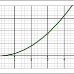
The point on the function where x = 3.

The third question–about finding the slope of a tangent line at x = 3–is our jumping off point into the mathematics of limits and calculus.

Some students do a single approximation–either forward or backward–, while others do both and take the average.

Finding the approximate slope using a forward difference.

The forward approximation involves finding the values for the function y = x2 at x = 3 and x = 4 and finding the slope between the two points:

  1. when x = 3, y = 9, so we have the point (x1,y1) = (3, 9)
  2. when x = 4, y = 16, so we have the point (x2,y2) = (3, 16)

The slope (m) between two points is found with the equation they learned back in algebra:

 \text{slope} = m = \frac{\Delta y}{\Delta x} = \frac{y_2-y_1}{x_2-x_1} = \frac{y_2-y_1}{\Delta x}

Where Δx = x2-x1 and Δy = y2-y1.

Using the two points above gives:

 \text{slope} = m = \frac{\Delta y}{\Delta x} = \frac{16-9}{4-3} = \frac{7}{1} = 7

Those who use the backward approximation simply use the point when x = 2 instead of x = 4, and they end up with a value for the slope of 5.

Averaging the forward and backward approximations give a slope of 6.

Now, since they know that the closer you make the points the better the approximation, I ask them to make a table to see what happens as they do so. This means reducing the value of Δx. In both the forward and backward approximation shown above, Δx = 1.

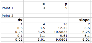
This can be done very quickly in Excel (or any other spreadsheet program), however, this time at least, most students chose to do it by hand. They end up with a table that looks like this:

y=x2-dx-to-zero

As dx gets smaller the calculated slope approaches 6.
As the difference in x gets smaller and approaches zero, the slope approaches 6.

As you plot slope versus the change in x (Δx), you can see that as Δx gets smaller and smaller and approaches zero, the slope gets closer and closer to 6. So we could say that:

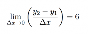
the limit of the slope as Δx approaches zero is 6.

Mathematically this can be written as:

limit-slope

or using the equation for slope:

limit-dx

Now, we can work on taking the limit in a more general way to do differentiation.

Introducing Limits (Calculus) with a Guitar

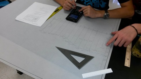
Creating the outline of a guitar.

One of the assigned tasks from last summer’s guitar building workshop was to create a few modules for use in class. I worked on an assignment that has students calculate the volume of a guitar body using trapezoidal approximation methods that can be a bridge between pre-calculus and calculus.

The first draft of this module is here: volume-activity-v01.pdf (the LaTeX file is volume-activity-v01.tex.zip ). It has made contact with the enemy students and the results have so far been very good.

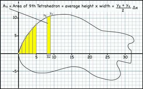
A method for finding the area of a guitar body by fitting trapezoids.

There were two things that I need to add for next time:

  1. How to find the area of a trapezoid: I should have some more detail about how I came up with the formula for calculating the area of each trapezoid (see the figure above). I multiply the average of the heights of the two sides of the trapezoid by the width of the base to get the area. Students tend to want to find the area of the lower rectangle, then add the area of the upper triangle. Their method gives the same answer for area, but results in a more complicated equation that takes more effort to generalize.
  2. Have them also find the slope of a tangent line to the outline of the guitar at a certain point. This assignment is intended to lead students up to the concept of limits with the idea that if you make the trapezoids thinner you’ll get less error in your calculation of the total area. So, as the width of the trapezoid approaches zero, you should get the exact area (with no error). The seemed to get that fairly well, however, when I get into the calculus, I actually first use limits to show them how to find derivatives of functions before I talk about finding areas under curves. As a result, I did ask the students to find the slope at a point on their guitar outline (I randomly chose a point from their outlines), and was very glad I did so. This should be included in the module.
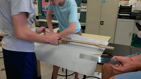
Students drawing trapezoids to fit the outline of the guitar, and calculating their areas.

Finally, in addition, I also showed them how to quickly calculate the trapezoid areas once they’d entered the coordinates of each point on their graphs into Excel. I did not test them on this afterward, so I’m not sure how much of it they absorbed.

The Final Product

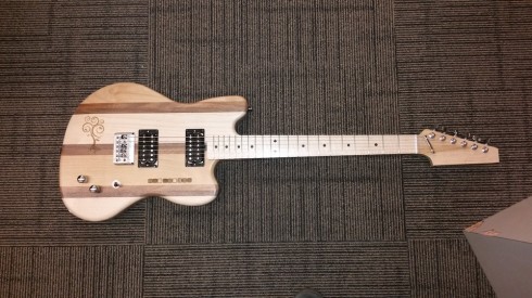
My electric guitar.
My electric guitar.

So I made the guitar. The guitarbuilding group make it hard to make a bad guitar, with the beautiful materials they provide, and their expert instruction, however, I’m inordinately proud of myself as well.

Indeed, as more and more of the elements fell into place over the course of the week, it really brought home the affective power of a) building something with your own hands, and b) the iconography of the electric guitar.

Now I have to figure out the logistics of doing this at Fulton. But as the workshop instructors pointed out, even if you don’t have students build one, just bringing the electric guitar into the classroom and saying, “Today we’re going to study sound,” really catches the attention.

Butterflies in Polar Coordinates

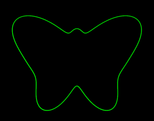
A butterfly outline drawn from a trigonometric function in polar coordinates.

I was looking for mathematical functions I could use to shape guitar bodies, and I came across Hubpages’ user calculus-geometry‘s beautiful page on how to generate butterfly outlines using functions in polar coordinates.

The butterfly above was generated using the function:

r(θ) = 12 – sin(θ) + 2 sin(3θ) + 2 sin(5θ) – sin(7θ) + 3 cos(2θ) – 2 cos(4θ)

The code I used (using VPython) is:

from visual import *

''' the main function '''
def r(theta):
    #r = 1+cos(theta)
    
    #Archimides' sprial
    #r = 0.5*(theta) 
    
    #heart: http://jwilson.coe.uga.edu/EMT669/Essay.ideas/Heart/Hearts.html
    #r = 5*sin(theta) - sin(5*theta)
    
    #butterfly: http://calculus-geometry.hubpages.com/hub/Butterfly-Curves-in-Polar-Coordinates-on-a-Graphing-Calculator
    #r = 8-sin(theta)+2*sin(3*theta)+2*sin(5*theta)-sin(7*theta)+3*cos(2*theta)-2*cos(4*theta)
    r = 12-sin(theta)+2*sin(3*theta)+2*sin(5*theta)-sin(7*theta)+3*cos(2*theta)-2*cos(4*theta)

    return r

'''convert to rectangular coordinates'''
def xy(r, theta):
    x = r * cos(theta)
    y = r * sin(theta)
    return vector(x, y)


path = curve(color=color.green, radius=.2)


theta = 0.0

print pi, theta, r(theta) , xy(r(theta), theta)

while theta <= 2*pi:
    rate(100)
    theta += 0.01
    path.append(pos=xy(r(theta), theta))


Sculpting the Guitar

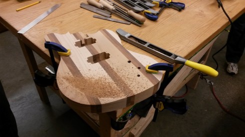
Sanding and sculpting the guitar bodies was loud, dusty and took a while.

Sculpting the guitar body.

The shape of an electric guitar’s body does not matter that much–they’ve even been made out of 2×4 (inches) pieces of wood–, so there’s a lot of room for creativity when sculpting your guitar’s shape. There’s a little more restriction for the guitar bodies from the guitarbuilding project because they come with cutouts for the electronics that have to be avoided. However, your main limitation is time.

Even with the big rasp, sculpting is not easy, especially since some of the types of wood used for the bodies can be quite hard. The darker strip in mine was particularly difficult.

I chose to carve out two parts of the body. First, it’s a lot more comfortable if the bit where the guitar tucks into your ribs is curved and smoothed; second, shaving down the area where your strumming forearm comes across the guitar makes the strings easier to get to.

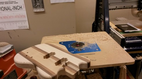
Once the sculpting was done, I used a router to round all the other edges.

Routing the edges with a table router.

Necks, Fretboards, and Scale Length

Pluck a string on a guitar and the sound you hear depends on how fast it vibrates. The frequency is how many times it vibrates back and forth in each second. An A4 note has a frequency of 440 vibrations per second (one vibration per second is one Hertz).

The vibration frequency of a guitar string depends on three things:

  • the mass of the string
  • the tension on the string (how tight it’s pulled)
  • and, the length of the string.

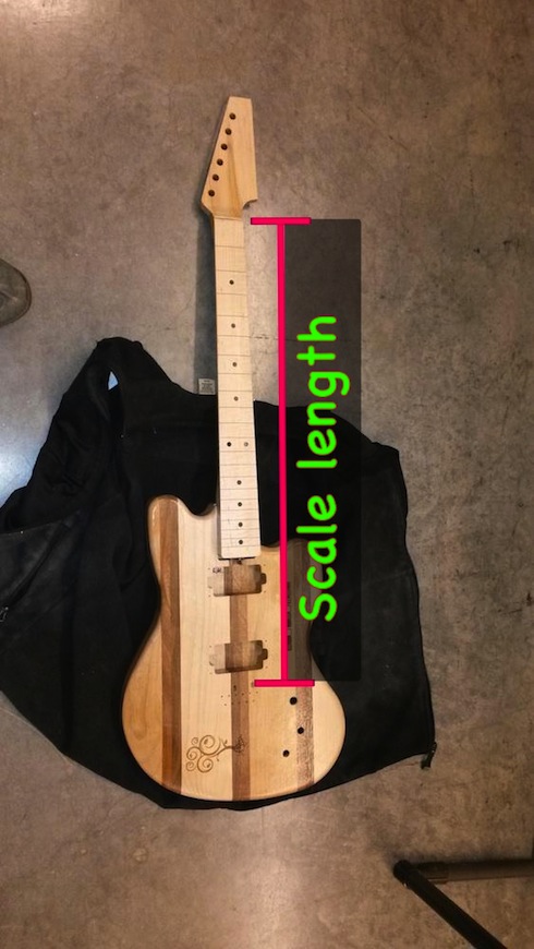
Guitar string sets come with wires of different masses. The guitar has little knobs on the end for adjusting the tension. For building the guitar, you have the most control over the last last parameter, the length of the string, which is called the scale length. Since the guitar string masses are pretty much set, and the strings can only hold so much tension, there are limits to the scale length you can choose for your guitar.

In a guitar, the scale length only refers to the length of the string that’s actually vibrating when you pluck the string, so it’s the distance between the nut and the bridge. For many guitars this turns out to be about 24.75 inches.

For a guitar, the scale length is the length of the strings that are free to vibrate.

Frets

To play different notes, you shorten the vibrating length of the string by using your finger to hold down the string somewhere along the neck of the instrument. The fret board (which is attached to the neck) has a set of marks to help locate the fingering for the different notes. How do you determine where the fret marks are located?

Well, the music of math post showed how the frequency of different notes are related by a common ratio (r). With:

 r = \sqrt[12]{2}

So given the notes:

Note Number (n) Note
0 C
1 C#
2 D
3 D#
4 E
5 F
6 F#
7 G
8 G#
9 A
10 A#
11 B
12 C

Since the equation for the frequency of a note is:

 f_n = f_0 \; r^n

we can find the length the string needs to be to play each note if we know the relationship between the frequency of the string (f) and the length of the string (l).

It turns out that the length is inversely proportional to the frequency.

 l = \frac{1}{f}

So we can calculate the length of string for each note (ln) as a fraction of the scale length (Ls).

 l_n = \frac{1}{f_n}

substituting for fn gives:

 l_n = \frac{1}{f_0 \; r^n}

but since we know the length for f0 is the scale length (Ls) (that inverse relationship again):

 l_n = \frac{1}{\frac{1}{L_s} \; r^n}

giving:

 l_n = \frac{L_s}{r^n}

When we play the different notes on the guitar, we move our fingers along the neck to shorten the vibrating parts of the string, so the base of the string stays at the same place–at the bridge. So, to mark where we need to place our fingers for each note, we put in marks at the right distance from the bridge. These marks are called frets, and we’ll call the distance from the bridge to each mark the fret distance (D_n). So we reformulate our formula to subtract the length of the vibrating string from the scale length of the guitar:

 D_n = L_s - \frac{L_s}{r^n}

Showing the fret distance.

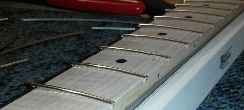
The fret marks are cut into a fret board that was supplied by the guitarbuilding team, which we glued onto the necks of our guitars. We did, however, have to add our own fret wire.

Placing the fret wire into the fret cuts. The wire still needs to be fully pressed in.

The team also has an activity for students to use a formula (a different one that’s recursive) to calculate the fret distance, but the Excel spreadsheet fret-spacing.xls can be used for reference (though it’s a good exercise for students to make their own).

The Math of Music

Mark French has an excellent YouTube channel on Mechanical Engineering, including the above video on Math and Music. The video describes the mathematical relationships between musical notes.

Given the sequence of notes: C, C#, D, D#, E, F, F#, G, G#, A, A#, B, C.

Let the frequency of the C note be f0, the frequency of C# be f1 etc.

The ratio of any two successive frequencies is constant (r). For example:

 \frac{f_1}{f_0} = r

so:

 \frac{f_1}{f_0} = \frac{f_2}{f_1} = \frac{f_4}{f_3} = \frac{f_{12}}{f_{11}} = r

We can find the ratio of the first and third notes by combining the first two ratios. First solve for f1 in the first equation:

 \frac{f_1}{f_0} = r

solving for f1,

 f_1 = f_0 \; r

now take the second ratio:

 \frac{f_2}{f_1} = r

and substitute for f1,

 \frac{f_2}{f_0 \; r} = r

which gives:

 \frac{f_2}{f_0} = r^2

We can now generalize to get the formula:

 \frac{f_n}{f_0} = r^n

or

 f_n = f_0 \; r^n

where,

  • n – is the number of the note

From this we can see that comparing the ratio of the first and last notes (f12/f0) is:

 \frac{f_{12}}{f_0} = r^{12}

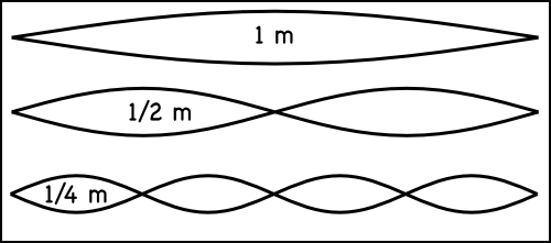
Now, as we’ve seen before, when we talked about octaves, the frequency of the same note in two different octaves is a factor of two times the lower octave note.

Click the waves to hear the different octaves. The wavelengths of the sounds are shown (in meters).


So, the frequency ratio between the first C (f0) and the second C (f12) is 2:

 \frac{f_{12}}{f_0} = 2

therefore:

 \frac{f_{12}}{f_0} = 2 = r^{12}

so we can now find r:

 r^{12} = 2

 r = \sqrt[12]{2}

Finally, we can now find the frequency of all the notes if we know that the international standard for the note A4 is 440 Hz.

Mark French has details on the math in his two books: Engineering the Guitar which is algebra based, and Technology of the Guitar, which is calculus based.