Calibration Curves for Salt (NaCl) Solutions

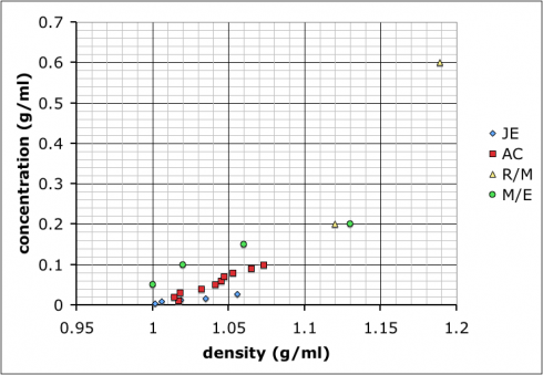
Calibration curves produced by different student groups to determine the relationship between density and concentration of salt (NaCl) solutions.

To start with chemistry class, we’re studying the properties of substances (like density) and how to measure and report concentrations. So, I mixed up four solutions of table salt (NaCl) dissolved in water of different concentrations, and put a drop of food coloring into each one to clearly distinguish them. The class as a whole had to determine the densities of the solutions, thus learning how to use the scales and graduated cylinders.

However, for the students interested in doing a little bit more, I asked them to figure out the actual concentrations of the solutions.

One group chose to evaporate the liquid and measure the resulting mass in the beakers. Others considered separating the salt electrochemically (I vetoed that one based on practicality.

Most groups ended up choosing to mix up their own sets of standard solutions, measure the densities of those, and then use that data to determine the densities of the unknown solutions. Their data is shown at the top of this post.

Finding the mass of solution in order to calculate its density.

The variability in their results is interesting. Most look like the result of systematic differences in making their measurements (different scales, different amounts of care etc.), but they all end up with curves where the concentration increases positively with density.

I showed the graph above to the class so we could talk about different sources of error, and how scientists will often compile the data from several different studies to get a better averaged result.

Then, I combined all the data and added a linear trend line so they could see how to do it using Excel (many of these students are in pre-calculus right now so it ties in nicely):
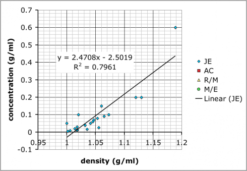
Trend line from combined data.

What we have not talked about yet–I hope to tomorrow–is how the R-squared value, which gives the goodness of the fit of the trend line to the data, is more a measure of precision rather than accuracy. It does say something about how internally consistent the data are, but not necessarily if the result is accurate.

It’s also useful to point out that the group with the best R-squared value is the one with only two data points because two data points will necessarily give a perfectly straight line. However, the groups that made more solutions might not have as good of an R-squared value, but, because of the multiple measurements, probably have more reliable results.

As for which group got the most accurate result: I added in some data I found by googling–it came off a UCSD website with no citation so I’m going to need to find a better reference. Comparing our data to the reference we find that team AC (the red squares) best match:
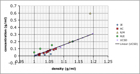
The straight line shows my (currently) accepted values for the concentration/density relationship.

Profits per Explosion: An application of Linear Regression

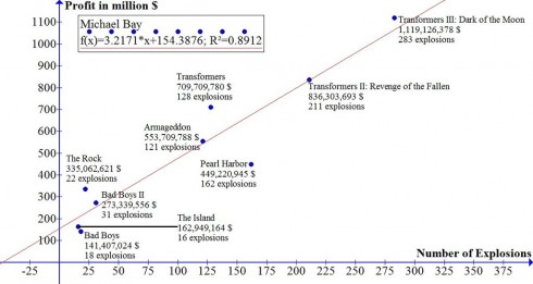
[Michael Bay] earns approximately 3.2 million $ for every explosion in his movies and a Michael Bay movie without explosions would earn 154.4 million $. This means that if Michael Bay wants to make a movie that earns more than Avatar’s 2781.5 million $ he has to have 817 explosions in his movie.

— Reddit:User:Mike-Dane: Math and Movies on Imgur.com.

There seems to be a linear relationship between the number of explosions in Michael Bay movies and their profitability. Graph by Reddit:User:Mike-Dane.

Reddit user Mike-Dane put together these entertaining linear regressions of a couple directors’ movie statistics. They’re a great way of showing algebra, pre-algebra, and pre-calculus students how to interpret graphs, and a somewhat whimsical way of showing how math can be applied to the fields of art and business.

Linear regression matches the best fit straight-line equations to data. The general equation for a straight line is:

y = mx + b

where m is the slope of the line — how fast in increases or decreases == and b is the intercept on the y-axis — which gives the initial value of the function.

So, for example, the Micheal Bay, profits vs. explosions, linear equation is:

Profit (in $millions) = 3.2 × (# of explosions) + 154

which means that a Michael Bay movie with no explosions (where # of explosions= 0) would make $154 million. And every additional explosion in a movie adds $3.2 million to the profits.

Furthermore, the regression coefficient (R2) of 0.89 shows that this equation is a pretty good match to the data.

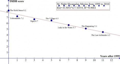
Mike-Dane gets an even better regression coefficient (R2 = 0.97) when he compares the quality of M. Night Shyamalan over time.

The scores of different M. Night Shyamalan movies calculated from user input on the Internet Movie DataBase (IMDB) decreases over time. Graph by Reddit:User:Mike-Dane.

In this graph the linear regression equation is:

Movie Score = -0.3014 × (year after 1999) + 7.8354

This equations suggests that the quality of Shyamalan’s movies decreases (notice the negative sign in the equation) by 0.3014 points every year. If you wanted to, you could, using some basic algebra, determine when he’d score a 0.

Warming of the West Antarctic Ice Sheet

… a breakup of the ice sheet, … could raise global sea levels by 10 feet, possibly more.

— Gillis (2012): Scientists Report Faster Warming in Antarctica in The New York Times.

In an excellent article, Justin Gillis highlights a new paper that shows the West Antarctic Ice sheet to be one of the fastest warming places on Earth.

The black star shows the Byrd Station. The colors show the number of melting days over Antarctica in January 2005. This number increases with warming temperatures (image from supplementary material in Bromwich et al., 2012).

Note to math students: The scientists use linear regression to get the rate of temperature increase.

The record reveals a linear increase in annual temperature between 1958 and 2010 by 2.4±1.2 °C, establishing central West Antarctica as one of the fastest-warming regions globally.

— Bromwich et al., (2012): Central West Antarctica among the most rapidly warming regions on Earth in Nature.

Momentum

A ball rolling down a ramp hits a car which moves off uphill. Can you come up with an experiment to predict how far the car will move if the ball is released from any height? What if different masses of balls are used?

Students try to figure out the relationship between the ball's release height and how far the car moves.

For my middle school class, who’ve been dealing with linear relationships all year, they could do this easily if the distance the car moves is directly proportional to height from which the ball was released?

The question ultimately comes down to momentum, but I really didn’t know if the experiment would work out to be a nice linear relationship. If you do the math, you’ll find that release height and the maximum distance the car moves are directly proportional if the momentum transferred to the car by the ball is also directly proportional to the velocity at impact. Given that wooden ball and hard plastic car would probably have a very elastic collision I figured there would be a good chance that this would be the case and the experiment would work.

It worked did well enough. Not perfectly, but well enough.