Numerical and Analytical Solutions 2: Constant Acceleration

Previously, I showed how to solve a simple problem of motion at a constant velocity analytically and numerically. Because of the nature of the problem both solutions gave the same result. Now we’ll try a constant acceleration problem which should highlight some of the key differences between the two approaches, particularly the tradeoffs you must make when using numerical approaches.

The Problem

  • A ball starts at the origin and moves horizontally with an acceleration of 0.2 m/s2. Print out a table of the ball’s position (in x) with time (every second) for the first 20 seconds.

Analytical Solution
We know that acceleration (a) is the change in velocity with time (t):

 a = \frac{dv}{dt}

so if we integrate acceleration we can find the velocity. Then, as we saw before, velocity (v) is the change in position with time:

 v = \frac{dx}{dt}

which can be integrated to find the position (x) as a function of time.

So, to summarize, to find position as a function of time given only an acceleration, we need to integrate twice: first to get velocity then to get x.

For this problem where the acceleration is a constant 0.2 m/s2 we start with acceleration:

 \frac{dv}{dt} = 0.2

which integrates to give the general solution,

 v = 0.2 t + c

To find the constant of integration we refer to the original question which does not say anything about velocity, so we assume that the initial velocity was 0: i.e.:

at t = 0 we have v = 0;

which we can substitute into the velocity equation to find that, for this problem, c is zero:

 v = 0.2 t + c
 0 = 0.2 (0) + c
 0 = c

making the specific velocity equation:
 v = 0.2 t

we replace v with dx/dt and integrate:

 \frac{dx}{dt} = 0.2 t
 x = \frac{0.2 t^2}{2} + c
 x = 0.1 t^2 + c

This constant of integration can be found since we know that the ball starts at the origin so

at t = 0 we have x = 0, so;

 x = 0.1 t^2 + c
 0 = 0.1 (0)^2 + c
 0 = c

Therefore our final equation for x is:

 x = 0.1 t^2

Summarizing the Analytical

To summarize the analytical solution:

 a = 0.2
 v = 0.2 t
 x = 0.1 t^2

These are all a function of time so it might be more proper to write them as:

 a(t) = 0.2
 v(t) = 0.2 t
 x(t) = 0.1 t^2

Velocity and acceleration represent rates of change which so we could also write these equations as:

 a(t) = \frac{dv}{dt} = 0.2
 v(t) = \frac{dx}{dt} = 0.2 t
 x(t) = x = 0.1 t^2

or we could even write acceleration as the second differential of the position:

 a(t) = \frac{d^2x}{dt^2} = 0.2
 v(t) = \frac{dx}{dt} = 0.2 t
 x(t) = x = 0.1 t^2

or, if we preferred, we could even write it in prime notation for the differentials:

 a(t) = x''(t) = 0.2
 v(t) = x'(t) = 0.2 t
 x(t) = x(t) =0.1 t^2

The Numerical Solution

As we saw before we can determine the position of a moving object if we know its old position (xold) and how much that position has changed (dx).

 x_{new} = x_{old} + dx

where the change in position is determined from the fact that velocity (v) is the change in position with time (dx/dt):

 v = \frac{dx}{dt}

which rearranges to:

 dx = v dt

So to find the new position of an object across a timestep we need two equations:

 dx = v dt
 x_{new} = x_{old} + dx

In this problem we don’t yet have the velocity because it changes with time, but we could use the exact same logic to find velocity since acceleration (a) is the change in velocity with time (dv/dt):

 a = \frac{dv}{dt}

which rearranges to:

 dv = a dt

and knowing the change in velocity (dv) we can find the velocity using:

 v_{new} = v_{old} + dv

Therefore, we have four equations to find the position of an accelerating object (note that in the third equation I’ve replaced v with vnew which is calculated in the second equation):

 dv = a dt
 v_{new} = v_{old} + dv
 dx = v_{new} dt
 x_{new} = x_{old} + dx

These we can plug into a python program just so:

motion-01-both.py

from visual import *

# Initialize
x = 0.0
v = 0.0
a = 0.2
dt = 1.0

# Time loop
for t in arange(dt, 20+dt, dt):

     # Analytical solution
     x_a = 0.1 * t**2

     # Numerical solution
     dv = a * dt
     v = v + dv
     dx = v * dt
     x = x + dx

     # Output
     print t, x_a, x

which give output of:

>>> 
1.0 0.1 0.2
2.0 0.4 0.6
3.0 0.9 1.2
4.0 1.6 2.0
5.0 2.5 3.0
6.0 3.6 4.2
7.0 4.9 5.6
8.0 6.4 7.2
9.0 8.1 9.0
10.0 10.0 11.0
11.0 12.1 13.2
12.0 14.4 15.6
13.0 16.9 18.2
14.0 19.6 21.0
15.0 22.5 24.0
16.0 25.6 27.2
17.0 28.9 30.6
18.0 32.4 34.2
19.0 36.1 38.0
20.0 40.0 42.0

Here, unlike the case with constant velocity, the two methods give slightly different results. The analytical solution is the correct one, so we’ll use it for reference. The numerical solution is off because it does not fully account for the continuous nature of the acceleration: we update the velocity ever timestep (every 1 second), so the velocity changes in chunks.

To get a better result we can reduce the timestep. Using dt = 0.1 gives final results of:

18.8 35.344 35.532
18.9 35.721 35.91
19.0 36.1 36.29
19.1 36.481 36.672
19.2 36.864 37.056
19.3 37.249 37.442
19.4 37.636 37.83
19.5 38.025 38.22
19.6 38.416 38.612
19.7 38.809 39.006
19.8 39.204 39.402
19.9 39.601 39.8
20.0 40.0 40.2

which is much closer, but requires a bit more runtime on the computer. And this is the key tradeoff with numerical solutions: greater accuracy requires smaller timesteps which results in longer runtimes on the computer.

Post Script

To generate a graph of the data use the code:

from visual import *
from visual.graph import *

# Initialize
x = 0.0
v = 0.0
a = 0.2
dt = 1.0

analyticCurve = gcurve(color=color.red)
numericCurve = gcurve(color=color.yellow)
# Time loop
for t in arange(dt, 20+dt, dt):

     # Analytical solution
     x_a = 0.1 * t**2

     # Numerical solution
     dv = a * dt
     v = v + dv
     dx = v * dt
     x = x + dx

     # Output
     print t, x_a, x
     analyticCurve.plot(pos=(t, x_a))
     numericCurve.plot(pos=(t,x))

which gives:
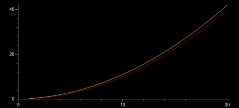
Comparison of numerical and analytical solutions using a timestep (dt) of 1.0 seconds.

Bending a Soccer Ball

Students from the University of Leicester have published a beautiful short research paper (pdf) on the physics of curving a soccer ball through the air.

It has been found that the amount a football bends depends linearly on the speed of the ball and the amount of spin.

— Sandhu et al., 2011: How to score a goal (pdf) in the University of Leicester’s Journal of Physics Special Topics

They derive the relationship from Bernoulli’s equation using some pretty straightforward algebra. The force (F) perpendicular to the ball’s motion that causes it to curl is:

F = 2 \pi R^3 \rho \omega v

and the distance the ball curls can be calculated from:

D = \frac{\pi R^3 \rho \omega}{ v m } x^2

where:

  • F = force perpendicular to the direction the ball is kicked
  • D = perpendicular distance the ball moves to the direction it is kicked (the amount of curl)
  • R = radius of the ball
  • ρ = density of the air
  • ω = angular velocity of the ball
  • v = velocity of the ball (in the direction it is kicked)
  • m = mass of the ball
  • x = distance traveled in the direction the ball is kicked

The paper itself is an excellent example of what a short, student research paper should look like. And there are number of neat followup projects that advanced, high-school, physics/calculus students could take on, such as: considering the vertical dimension — how much time it take for the ball to rise and fall over the wall; creating a model (VPython) of the motion of the ball; and adding in the slowing of the ball due to air friction.

ScienceDaily

Draining a Bottle Part 2: Linearizing Equations when you have to

Yesterday we used calculus to find the equation for the height of water in a large plastic water bottle as the water drained out of a small hole in the bottom.

Perhaps the most crucial point in the procedure was fitting a curve to the measured reduction of the water’s outflow rate over time. Yesterday, in our initial attempt, we used a straight line for the curve, which produced a very good fit.

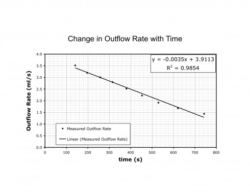
Figure 1. The change in the outflow rate over time can be well approximated by a straight line.

The R2 value is a measure of how good a fit the data is to the trendline. The straight line gives an R2 value of 0.9854, which is very close to a perfect fit of 1.0 (the lowest R2 can go is 0.0).

The resulting equation, written in terms of the outflow rate (dV/dt) and time (t), was:

 \frac{dV}{dt} = -0.0035 t + 3.9113

However, if you look carefully at the graph in Figure 1, the last few data points suggest that the outflow does not just linearly decrease to zero, but approaches zero asymptotically. As a result, a different type of curve might be a better trendline.

Types of Equations

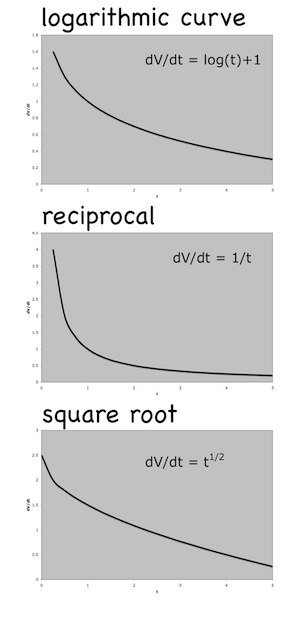
So my calculus students and I, with a little help from the pre-Calculus class, tried to figure out what types of curves might work. There are quite a few, but we settled for looking at three: a logarithmic function, a reciprocal function, and a square root function. These are shown in Figure 2.

Figure 2. Example curves that might better describe the relationship between outflow and time.

I steered them toward the square root function because then we’d end up with something akin to Torricelli’s Law (which can be derived from the physics). A basic square root function for outflow would look something like this:

 \frac{dV}{dt} = a \sqrt{t} + b

the a coefficient stretches the equation out, while the b coefficient moves the curve up and down.

Fitting the Curve

Having decided on a square-root type function, the next problem was trying to find the actual equation. Previously, we used Excel to find the best fit straight line. However, while Excel can fit log, exponential and power curves, there’s no option for fitting a square-root function to a graph.

To get around this we linearized the square-root function. The equation, after all, looks a lot like the equation of a straight line already, the only difference is the square root of t, so let’s substitute in:

 x = \sqrt{t}

to get:

 \frac{dV}{dt} = a x + b

Now we can get Excel to fit a straight line to our data, but we have to plot the square-root of time versus temperature instead of the just time versus temperature. So we take the square root of all of our time measurements:

Time Square root of time Outflow rate
t (s) t1/2 = x (s1/2) dV/dt (ml/s)
0.0 0 3.91
45.5 6.75 3.52
97.8 9.89 2.94
140.9 11.87 3.52
197 14.04 3.21
257 16.05 3.01
315.1 17.75 2.81
380.1 19.50 2.53
452.9 21.28 2.23
529.6 23.01 1.92
620.7 24.91 1.69
742.7 27.25 1.45

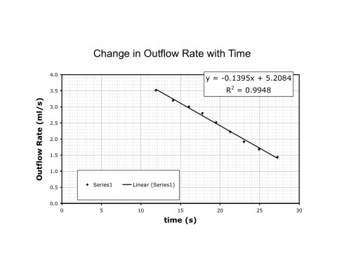
We can now plot the outflow rate versus the square root of time (Figure 3).

Figure 3. Linear trend relating the outflow rate to the square root of time. The regression coefficient (R2) of 0.9948 is better than the simply linear trend of outlfow rate versus time (which was 0.9854).

The equation Excel gives (Figure 3), is:

 \frac{dV}{dt} = -0.1395 x + 5.21

and we can substitute back in for x=t1/2 to get:

 \frac{dV}{dt} = -0.1395 \sqrt{t} + 5.21

Getting back to the Equation for Height

Now we can do the same procedure we did before to find the equation for height.

First we substitute in V=πr2h:

 \frac{d(\pi r^2 h}{dt} = -0.1395 \sqrt{t} + 5.21

Factor out the πr2 and move it to the other side of the equation to solve for the rate of change of height:

 \frac{dh}{dt} = \frac{-0.1395}{\pi r^2} \sqrt{t} + \frac{5.21}{\pi r^2}

Then integrate to find h(t) (remember \sqrt{t} = t^{1/2} ) :

 \int \frac{dh}{dt} dt = \int \left( \frac{-0.1395}{\pi r^2} t^{1/2} + \frac{5.21}{\pi r^2} \right) dt

gives:

 h =  \frac{-0.1395}{(3/2) \pi r^2} t^{3/2} + \frac{5.21}{\pi r^2} t + c

which might look a bit ugly, but that’s only because I haven’t simplified the fractions. Since the radius (r) is 7.5 cm:

 h =  -0.000526 t^{3/2} + 0.029 t + c

Finally we substitute in the initial value (t=0, h=11) to solve for the coefficient:

 c = 11

giving the equation:

 h =  -0.000526 t^{3/2} + 0.029 t + 11

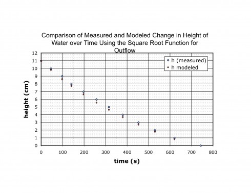
Plotting the equations shows that it matches the measured data fairly well, although not quite as well as when we used the previous linear function for outflow.

Figure 4. Integrating a square root function for the outflow rate gives a modeled function for the changing height over time that slightly undermatches the measured heights.

Discussion

I’m not sure why the square root function for outflow does not give as good a match of the measurements of height as does the linear function, especially since the former better matches the data (it has a better R2 value).

It could be because of the error in the measurements; the gradations on the water bottle were drawn by hand with a sharpie so the error in the height measurements there alone was probably on the order of 2-3 mm. The measurement of the outflow volume in the beaker was also probably off by about 5%.

I suspect, however, that the relatively short time for the experiment (about 15 minutes) may have a large role in determining which model fit better. If we’d run the experiment for longer, so students could measure the long tail as the water height in the bottle got close to the outlet level and the outflow rate really slowed down, then we’d have found a much better match using the square-root function. The linear match of the outflow data produces a quadratic equation when you integrate it. Quadratic equations will drop to a minimum and then rise again, unlike the square-root function which will just continue to sink.

Conclusions

The linearization of the square-root function worked very nicely. It was a great mathematical example even if it did not produce the better result, it was still close enough to be worth it.

The Draining of a Plastic Bottle: Integrating a Physics Experiment into Calculus

Abstract

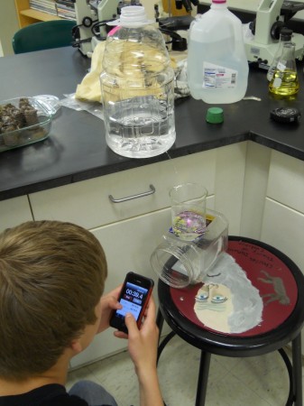
I punched a small hole (about 1mm radius) in a one gallon plastic bottle and had my students measure the rate at which water drained. Even though the apparatus and measurement technique was fairly rough, we were able to, with a little calculus, determine the equation for the height of the water in the bottle as a function of time.

Figure 1. A student uses a stopwatch to measure the outflow rate of water from the plastic bottle.

Introduction

Questions about water draining from a tank are a pretty common in calculus textbooks, but there is a significant difference between seeing the problem written down, and having to figure it out from a physical example. The latter is much more challenging because it does not presuppose any relationships for the change in the height of water with time; students must determine the relationship from the data they collect.

The experimental approach mimics the challenges faced by scientists such as Henry Darcy who first determined the formulas for groundwater flow (Darcy, 1733) almost 300 years ago, not long after the development of modern calculus by Newton and Leibniz (O’Conner and Robertson, 1996).

Procedure

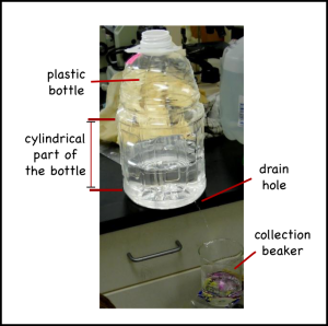
Figure 2. The apparatus.

I punched a small hole, about 1mm in radius, in the base of a plastic, one-gallon bottle. I chose this particular type of bottle because the bulk of it was cylindrical in shape.

Students were instructed to figure out how the rate at which water flowed out (outflow rate) changed with time, and how the height of the water (h) in the bottle changed with time. These relationships would allow me to predict the outflow rate at any time, as well as how much water was left in the container at any time.

Data collection:

  1. To measure height versus time, we marked the side of the bottle (within the cylindrical region) in one centimeter increments and recorded the time it took for the water level to drop from one mark to the next. There were a total of 11 marks.
  2. To measure the outflow rate, we intercepted the outflow using a 25 ml beaker (not shown in Figure 2), and measured the time it took to fill to the 25 ml mark.

Results

Time elapsed since last measurement Height of water in container Time to fill 25ml beaker
Δt (s) h (cm) tf (s)
0.0 11 6.4
45.5 10 7.1
52.3 9 8.5
43.1 8 7.1
56.1 7 7.8
60.6 6 8.3
57.6 5 8.9
65.0 4 9.9
72.8 3 11.2
76.7 2 13.0
91.1 1 14.8
122.0 0 17.3

Table 1: Outflow rate, water height change with time.

To analyze the data, we calculated the total time (the cumulative sum of the elapsed time since the previous measurement) and the outflow rate. The outflow rate is the change in volume with time:

 \text{outflow rate} = \frac{volume}{time} = \frac{dV}{dt} = \frac{25 ml}{t_f}

So our data table becomes:

Time Height of water in container Outflow rate
t (s) h (cm) dV/dt (ml/s)
0.0 11 3.91
45.5 10 3.52
97.8 9 2.94
140.9 8 3.52
197 7 3.21
257 6 3.01
315.1 5 2.81
380.1 4 2.53
452.9 3 2.23
529.6 2 1.92
620.7 1 1.69
742.7 0 1.45

Table 2. Height of water and outflow rate of the bottle.

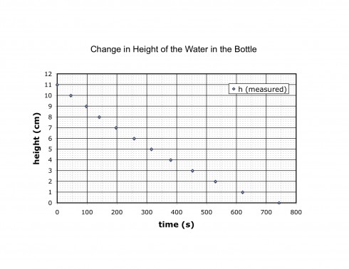
The graph of the height of the water with time shows a curve, although it is difficult to determine precisely what type of curve. My students started by trying to fit a quadratic equation to it, which should work as we’ll see in a minute.

Figure 3. The decrease in height with time is not a straight line (is non-linear).

The plot of the outflow rate versus time, however, shows a pretty good linear trend. (Note that we do not use the first three datapoints (in Table 2), which we believe are erroneous because we were still sorting out the measuring method.)

Although I’ll note here that the data should ideally be modeled using a square root equation (Torricelli’s Law), that is beyond the present scope of the problem (we’ll try that tomorrow as a follow exercise).

Plotting the data in Excel we could add a linear trendline.

Figure 4. The outflow rate decreases linearly with time.

For the linear trendline, Excel gives the equation:

 y = -0.0035 x + 3.9113

The y-axis is outflow rate (the change in volume with time), and the x axis is time (t), so the linear equation becomes:

 \frac{dV}{dt} = -0.0035 t + 3.9113

Notice that this is a differential equation.

To determine the rate of at which the height of water in the container is changing, we need to recognize that the container is cylindrical in shape, and the volume (V) of a cylinder depends on its radius (r) and height (h):

 V = \pi r^2 h

which can be substituted into differential in the rate equation:

 \frac{d(\pi r^2 h)}{dt} = -0.0035 t + 3.9113

since π and the radius (r) are constants (since the jug’s shape is a cylinder), they can be pulled out of the differential:

 \pi r^2 \frac{dh}{dt} = -0.0035 t + 3.9113

Dividing through by πr2 solves for the rate of change of height:

  \frac{dh}{dt} = \frac{-0.0035 t + 3.9113}{\pi r^2}

Isolating the coefficients gives:

  \frac{dh}{dt} = \frac{-0.0035}{\pi r^2} t + \frac{3.9113}{\pi r^2}

This equation should give the rate at which the height changes with time, however, if you look at it carefully you’ll realize that for the time range we’re using (less than 800 seconds) the value of dh/dt will always be positive. We correct this by recognizing that the outflow rate is a loss of water, so a positive outflow should result in a negative change in height, therefore we rewrite the equation as:

  -\frac{dh}{dt} = \frac{-0.0035}{\pi r^2} t + \frac{3.9113}{\pi r^2}

which gives:

  \frac{dh}{dt} = \frac{0.0035}{\pi r^2} t - \frac{3.9113}{\pi r^2}

Now comes the calculus

Now, we can use this rate equation to find the equation for height versus time by integrating with respect to time:

  \int \frac{dh}{dt} dt = \int \left( \frac{0.0035}{\pi r^2} t - \frac{3.9113}{\pi r^2} \right) dt

to get:

 h = \frac{0.0035}{2 \pi r^2} t^2 - \frac{3.9113}{\pi r^2} t + c

And all we have to do to the find the constant of integration is substitute in a known point, an initial value. As is often the case, the best point to use is the starting point where t=0 makes the rest of the calculations easier. In our case, when t=0, h=11:

 11 = \frac{0.0035}{2 \pi r^2} (0)^2 - \frac{3.9113}{\pi r^2} (0) + c

so:

 c = 11

And our final equation becomes:

 h = \frac{0.0035}{2 \pi r^2} t^2 - \frac{3.9113}{\pi r^2} t + 11

which is a quadratic equation as my students guessed before we did the calculus.

Does it work?

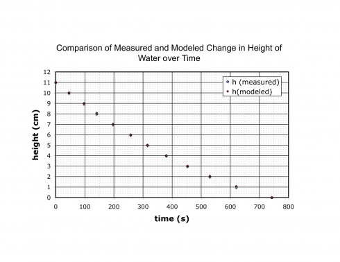
You will notice that in the math above, we never use the height data in determining equation for height versus time; all the calculations are based on the trendline for the outflow rate versus time.

As a result, we can compare the results of our equation to the actual measurements to see if our calculations are even close. Remarkably, they are.

Figure 5. The results from our equation (modeled) match the measured heights so well, the data points are difficult to distinguish on the graph.

Discussion

Despite all the potential for error, particularly, our relatively crude measurement techniques, and the imperfect cylindrical shape of our plastic bottle, the experiment went remarkably well.

Students found it quite challenging, and required some assistance even though this is a problem they have seen before in their textbook.

The problems in the textbook use Torricelli’s Law, which should much better describe the draining of a tank than the linear equation we find for dV/dt.

Torricelli’s Law:

 \frac{dV}{dt} = a \sqrt{2gh}

where a is the area of the outlet hole, and g is the acceleration due to gravity.

In our actual experiment it is difficult to tell that a square root function would work better. Excel does not have an option for matching a square root function, so the calculations would become more involved (although it could be set up using Excel’s iterative solver or Goal Seek function).

Conclusion

Our experiment to use calculus to determine the rate of change of the height of water in a leaking plastic water bottle was a successful exercise even though the roughness of the data collection did not permit identification of the square root law for leakage.