Programming Agents

An artful spaceship.

For my programming elective, I thought I’d try to get students programming autonomous agents that we could all compile together into some type of game. Since it was, for most of them a first class in programming, this has proven a little too ambitious, and I’ve had to adjust a bit to build up to it.

Step 1: Build a spaceship/vehicle/agent.
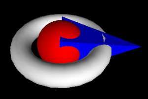
A simple ship made of a sphere, ring, and pyramid, with a clear front end (pointed to the left: vector=(1,0,0).
  • We’re using VPython so we can build 3d ships. Students get to exercise their creativity a bit and learn how to place things in 3d co-ordinate space.
  • The ship must have a front end and all the parts must be put into a single frame so the whole thing can be moved as a unit.
  • Although it’s not required, I’ve added in the beginnings of a trail so we can track the motion of the spaceship
from visual import *

f = frame()
r = ring(frame=f, thickness=.25, axis=(0,1,0))
cabin = sphere(frame=f, radius=0.6, color=color.red)
front = pyramid(frame=f, height=1,width=1,length=2, color=color.blue)
trail = curve(pos=[f.pos,])

Step 2: Make the spaceship a class.

  • Putting the spaceship in a separate class, away from the rest of the code, makes it easier to move from one program to another. That means we can import everyone’s ships into a single program at the end.
from visual import *

class spaceship1:

    def __init__(self):

        self.f = frame()
        self.r = ring(frame=self.f, thickness=.25, axis=(0,1,0))
        self.cabin = sphere(frame=self.f, radius=0.6, color=color.red)
        self.front = pyramid(frame=self.f, height=1,width=1,length=2, color=color.blue)
        self.trail = curve(pos=[self.f.pos,])

ss = spaceship1()

Make the spaceship move

  • We’re going to control the movement of the spaceship using the arrow keys. Left and right to turn; up and down to accelerate and decelerate.
  • To allow movement, we’ll put the keyboard controls into an infinite loop, but to allow maximum flexibility (and to show how to use create methods in a class) we’re putting the actual movement in as methods in the class: the turning method is named turn_xz and movement is move_xz since all the motion is going to be restricted in the xz plane for now.
from visual import *

class spaceship1:

    def __init__(self):

        self.f = frame()
        self.r = ring(frame=self.f, thickness=.25, axis=(0,1,0))
        self.cabin = sphere(frame=self.f, radius=0.6, color=color.red)
        self.front = pyramid(frame=self.f, height=1,width=1,length=2, color=color.blue)
        self.trail = curve(pos=[self.f.pos,])

    def turn_xz(self, turn_rate):
        self.f.axis = rotate(self.f.axis, turn_rate, (0,1,0))

    def move_xz(self, speed):
        self.f.pos = self.f.pos + self.f.axis*speed
        self.trail.append(pos=self.f.pos)
                          
ss = spaceship1()
turn = 0.0
speed=0.0

while 1:
    rate(20)  #slows down execution of the loop

    ss.turn_xz(turn)
    ss.move_xz(speed)

    if scene.kb.keys: # event waiting to be processed?
        s = scene.kb.getkey() # get keyboard info

        if s == 'left':
            turn = turn + 0.01
        if s == 'right':
            turn = turn - 0.01

        if s == 'up':
            speed = speed + 0.01
        if s == 'down':
            speed = speed - 0.01

        if s == ' ':
            if turn <> 0:
                turn = 0
            elif speed <> 0:
                speed = 0

Fire missiles

  • We add in missiles by creating a class very similar to the spaceship. For now our missile is just a ball but I’m putting it into a frame anyway in case later on I want it to be a composite object.
  • Since we can fire multiple missiles, in the code I create a list to hold all the missiles.
  • Missiles are fired using the “a” key.
from visual import *

class spaceship1:

    def __init__(self):

        self.f = frame()
        self.r = ring(frame=self.f, thickness=.25, axis=(0,1,0))
        self.cabin = sphere(frame=self.f, radius=0.6, color=color.red)
        self.front = pyramid(frame=self.f, height=1,width=1,length=2, color=color.blue)
        self.trail = curve(pos=[self.f.pos,])

    def turn_xz(self, turn_rate):
        self.f.axis = rotate(self.f.axis, turn_rate, (0,1,0))

    def move_xz(self, speed):
        self.f.pos = self.f.pos + self.f.axis*speed
        self.trail.append(pos=self.f.pos)
          
class missile:
    def __init__(self, axis, pos):

        self.f = frame(axis=axis, pos=pos)
        self.r = sphere(frame=self.f, radius=0.2, color=color.green)
        self.speed = 0.5
        

    def move_xz(self):
        self.f.pos = self.f.pos + self.f.axis*self.speed

                
ss = spaceship1()
turn = 0.0
speed=0.0

missiles = []  #list for missiles

while 1:
    rate(20)  #slows down execution of the loop

    ss.turn_xz(turn)
    ss.move_xz(speed)

    #move missiles
    for i, m in enumerate(missiles):
        m.move_xz()

    if scene.kb.keys: # event waiting to be processed?
        s = scene.kb.getkey() # get keyboard info

        if s == 'left':
            turn = turn + 0.01
        if s == 'right':
            turn = turn - 0.01

        if s == 'up':
            speed = speed + 0.01
        if s == 'down':
            speed = speed - 0.01

        if s == ' ':
            if turn <> 0:
                turn = 0
            elif speed <> 0:
                speed = 0

        #fire missile
        if s == 'a':
            missiles.append(missile(ss.f.axis, ss.f.pos))

Final adjustments

  • Finally, I’m going to put in a boundary, and set it up to delete the missiles if they go out of bounds.
  • I’m also going to set an option so that the scene follows the ship, which makes it easier to keep track of things.
from visual import *

class spaceship1:

    def __init__(self):

        self.f = frame()
        self.r = ring(frame=self.f, thickness=.25, axis=(0,1,0))
        self.cabin = sphere(frame=self.f, radius=0.6, color=color.red)
        self.front = pyramid(frame=self.f, height=1,width=1,length=2, color=color.blue)
        self.trail = curve(pos=[self.f.pos,])

    def turn_xz(self, turn_rate):
        self.f.axis = rotate(self.f.axis, turn_rate, (0,1,0))

    def move_xz(self, speed):
        self.f.pos = self.f.pos + self.f.axis*speed
        self.trail.append(pos=self.f.pos)
                          

class missile:
    def __init__(self, axis, pos):

        self.f = frame(axis=axis, pos=pos)
        self.r = sphere(frame=self.f, radius=0.2, color=color.green)
        self.speed = 0.5
        

    def move_xz(self):
        self.f.pos = self.f.pos + self.f.axis*self.speed

class bounds:
    def __init__(self, boundary_distance):
        self.boundary_distance = boundary_distance
        self.border = curve(pos=[(-boundary_distance,0,-boundary_distance),
                                 (boundary_distance,0,-boundary_distance),
                                 (boundary_distance,0,boundary_distance),
                                 (-boundary_distance,0,boundary_distance),
                                 (-boundary_distance,0,-boundary_distance)])
    def in_bounds(self, pos):
        if ( pos.x < -self.boundary_distance or
             pos.x > self.boundary_distance or
             pos.z < -self.boundary_distance or
             pos.z > self.boundary_distance):
            return false
        else:
            return true
        

ss = spaceship1()
turn = 0.0
speed=0.0
l_track_ship = 1
scene.range=10
scene.forward = (0,-1,0)
missiles = []

boundary_distance = 100
boundary = bounds(boundary_distance)

while 1:
    rate(20)

    if l_track_ship > 0:
        scene.center = ss.f.pos
    
    ss.turn_xz(turn)
    ss.move_xz(speed)

    #move missiles
    del_list = []
    for i, m in enumerate(missiles):
        m.move_xz()

        #delete missile if out of bounds
        if boundary.in_bounds(m.f.pos) == False:
            del_list.append(i)
    for i in del_list:
        missiles[i].f.visible = False
        del missiles[i]
            
    
    #if m <> None:
    #    m.move_xz()

    if scene.kb.keys: # event waiting to be processed?
        s = scene.kb.getkey() # get keyboard info

        if s == 'left':
            turn = turn + 0.01
        if s == 'right':
            turn = turn - 0.01

        if s == 'up':
            speed = speed + 0.01
        if s == 'down':
            speed = speed - 0.01

        if s == ' ':
            if turn <> 0:
                turn = 0
            elif speed <> 0:
                speed = 0

        #fire missile
        if s == 'a':
            missiles.append(missile(ss.f.axis, ss.f.pos))
    

Next steps

Now that we’re cooking with charcoal — we have a functioning program — the next steps will be setting up a target to shoot at, and, if the students are ready, letting them program their ships to move autonomously. If they’re not ready then, as an example, I’ll program some opposition.

Learning Matricies by Programming a Matrix Solver

One of my pre-Calculus students convinced me that the best way for him to learn how to work with matrices was for him to program a matrix solver. I helped him create a Gaussian Elimination solver in Python (which we’ve been using since last year).

Gaussian Elimination Matrix Solver by Alex Shine (comments by me).

from visual import *

'''The coefficient matrix (m) can be any sized square matrix 
   with an additional column for the solution'''
m = [ [1,-2,1,-4],[0,1,2,4],[2,3,-2,2]]

'''Convert the input matrix, m (which is a list) into an array'''
a = array(m,float)
print "Input matrix:"
print a
print

'''Get the shape of the matrix (number of rows and columns)'''
(r,c) = a.shape 

rs = (1-r)

'''Solve'''
for j in range(r):

    print "Column #:", j
    for i in range(r):
        if a[i,j] <> 0:
            a[i,:] = a[i,:] / a[i,j]
    print a
    print

    for i in range(rs+j,j):
        if a[i,j] <> 0:
            a[i,:] = a[j,:] - a[i,:]
    print a
    print

print "Solution"
for i in range (r):
    a[i,:] = a[i,:] / a[i,i]
    print "Variable", i, "=", a[i,-1]

print
print "Solution Matrix:"
print a

The code above solves the following system of equations:


  x - 2y +  z = -4 
       y + 2z =  4 
 2x + 3y - 2z =  2 

Which can be written in matrix form as such:

 \left[ \begin{array}{ccc} 1 & -2 & 1 \\ 0 & 1 & 2 \\ 2 & 3 & -2 \end{array} \right]  \left[ \begin{array}{c} x \\ y \\ z \end{array} \right] =  \left[ \begin{array}{c} -4 \\ 4 \\ 2 \end{array} \right]

You use the solver by taking the square matrix on the left hand side of the equation and combining it with the column on the hand side as an additional column:

 \left[ \begin{array}{cccc} 1 & -2 & 1 & -4 \\ 0 & 1 & 2 & 4\\ 2 & 3 & -2 & 2\end{array} \right]

This is entered into the program as the line:

m = [ [1,-2,1,-4],[0,1,2,4],[2,3,-2,2]]

When you run the above program you should get the results:

>>> ================================ RESTART ================================
>>> 
Input matrix:
[[ 1. -2.  1. -4.]
 [ 0.  1.  2.  4.]
 [ 2.  3. -2.  2.]]

Column #: 0
[[ 1.  -2.   1.  -4. ]
 [ 0.   1.   2.   4. ]
 [ 1.   1.5 -1.   1. ]]

[[ 1.  -2.   1.  -4. ]
 [ 0.   1.   2.   4. ]
 [ 0.  -3.5  2.  -5. ]]

Column #: 1
[[-0.5         1.         -0.5         2.        ]
 [ 0.          1.          2.          4.        ]
 [-0.          1.         -0.57142857  1.42857143]]

[[ 0.5         0.          2.5         2.        ]
 [ 0.          1.          2.          4.        ]
 [ 0.          0.          2.57142857  2.57142857]]

Column #: 2
[[ 0.2  0.   1.   0.8]
 [ 0.   0.5  1.   2. ]
 [ 0.   0.   1.   1. ]]

[[-0.2  0.   0.   0.2]
 [ 0.  -0.5  0.  -1. ]
 [ 0.   0.   1.   1. ]]

Solution
Variable 0 = -1.0
Variable 1 = 2.0
Variable 2 = 1.0

Solution Matrix:
[[ 1. -0. -0. -1.]
 [-0.  1. -0.  2.]
 [ 0.  0.  1.  1.]]
>>>

Be aware that:

  • The code is designed to take any size of matrix.
  • The matrix you put in can not have any zeros on its diagonal, so some manipulation is often necessary before you can use the code.

Other notes:

  • The negative zeros (-0) that show up especially in the solution matrix may not look pretty but do not affect the solution.
  • The code imports the vpython module in the first line but what it really needs is the numpy module, which vpython imports, for the arrays.

The next step is to turn this into a function or a class that can be used in other codes, but it’s already proved useful. My calculus students compared their solutions for the coefficients of a quadratic equation that they had to solve for their carpet friction experiment, which was great because their first answers were wrong.

A calculus student uses the matrix solver. Mr. Shine is now trying to convert the solver into an iPhone app.

Concave Mirror Ray Diagrams in VPython

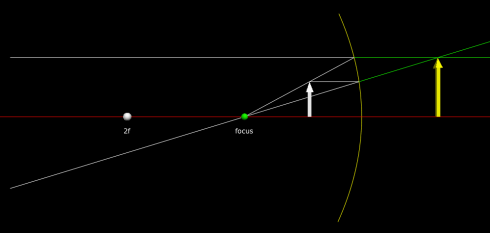
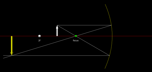
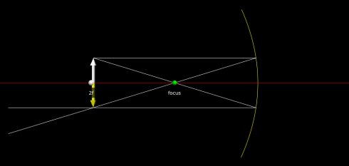
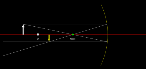
I put together a VPython model to interactively illustrate how ray diagrams can be used to determine the appearance of an object in a concave, parabolic mirror. The video below demonstrates, but the code can be found here.

The white arrow is the object, and the yellow arrow shows it apparent magnification and orientation. You can drag the arrow around by its base, or make it taller (or shorter) by dragging the tip of the arrow up and down.

Summary of Appearance

When the object is closer to the mirror than the mirror’s focal distance then the object appears enlarged.

Enlarged when close.

When the object is between 1 and 2 focal distances away from the lens, it still appears enlarged, but is upside down. (Note that at one focal distance away the object disappears entirely from the mirror.)

When the object is between 1 and 2 focal distances away from the lens, it still appears enlarged, but is upside down.

At twice the focal distance the object appears to be the same size but upside down.

At twice the focal distance the object appears to be the same size but upside down.

Beyond 2 times the focal distance the object appears upside down and shrunken.

Beyond 2 times the focal distance the object appears upside down and shrunken.

NOTE: To create images from VPython, and then convert them into a movie, I used this technique.

A Study in Linear Equations

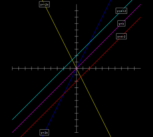
The effects of changing the constants in the equation of a line (y=mx+b). Image by Tess R.

My high school pre-Calculus class is studying the subject using a graphical approach. Since we’re half-way through the year I thought it would be useful to introduce some programming by building their own graphical calculators using Vpython.

Now, they all have graphical calculators, and Vpython does have its own graphing capabilities, but they’re fairly simple, only 2-dimensional, and way too automatic, so I prefer to have students program the calculators in full 3d space.

My approach to graphing is fairly simple too, but its nice because it introduces:

  • Co-ordinates: Primarily in 2d (co-ordinate plane), but 3d is easy;
  • Lists: in this case its a list of coordinates on a line;
  • Loops: (specifically for loops) to repeat actions and produce a sequence of numbers (with range); and
  • A sideways glance at matrix-like operations with arrays: A list of numbers can be treated like a matrix in some relatively simple circumstances. However, it’s not real matrix operations: multiplying a scalar by a list works like real matrix multiplication, but multiplying two lists multiplies the corresponding elements in the list.

A Simple Graphing Program

Start the program with the standard vpython header:

from visual import *

x and y axes: curves and lists

Next create the x and y axes. This introduces the curve object and lists, because Vpython draws its curve from a series of points held in a list.

To keep things simple, we’re letting the graph go from -10 to positive 10 along both axes, which makes the x-axis a line segment with only two points:

line_segment = [(-10,0), (10,0)]

The square brackets say that what’s inside as a list. In this case it’s a list of two coordinate pairs, (-10,0) and (10,0).

Now we create a line using Vpython’s curve and tell it that the positions of the points on the curve are the ones we just defined:

xaxis = curve(pos=line_segment)

To create the y-axis, we do the same thing but change the coordinate pair to (0,-10) and (0,10).

line_segment = [(0,-10),(0,10)]
yaxis = curve(pos=line_segment)

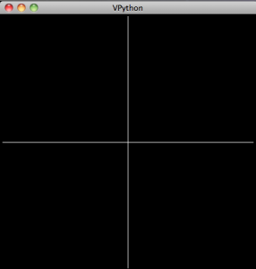
Which should produce:

Very simple x and y axes.

Tic-marks: loops

In order to be better able to keep track of things, we’ll need some tic-marks on the axes. Ideally we’d like to label them too, but I think it works well enough to save that for later.

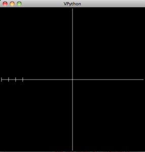
I start by having students create the first few tic-marks and then look for the emerging pattern. Their first attempts usually look something like this:

mark1 = curve(pos=[(-10,0.3),(-10,-0.3)])
mark2 = curve(pos=[(-9,0.3),(-9,-0.3)])
mark3 = curve(pos=[(-8,0.3),(-8,-0.3)])
mark4 = curve(pos=[(-7,0.3),(-7,-0.3)])
A few tic marks.

However, instead of tediously writing out these lines we can automate it by noticing that the only things that change are the x-coordinate of the coordinate pairs: they go from -10, to -9, to -8 etc.

So we want to produce a set of numbers that go from -10 to 10, in increments of 1, and use those number to make the tic-marks. The range function will do just that: specifically, range(-10,10,1). Actually, this list only goes up to 9, but that’s okay for now.

We tell the program to go through each item in the list and give its value to the variable i using a for loop:

for i in range(-10,10,1):
    mark = curve(pos=[(i,0.3),(i,-0.3)])

In python, everything indented after the for statement is within the loop.

Tic marks on the x-axis.

The y-axis’ tic-marks are similar, and its a nice little challenge for students to figure them out. They usually come up with a separate loop, eventually, that looks something like:

for i in range(-10,10,1):
    mark = curve(pos=[(0.3, i),(-0.3,i)])
Our axes.

The Curve

Now to create a line we really only need two points. However, so that we can make other types of curves later on we’ll create a line with a series of points. We’ll create the x and y values separately:

First we set up the set of x values:

line = curve(x=arange(-10,10,0.1))

Note that I use the arange function which is just like the range function but gives you decimal values (so you can do fractions) instead of just integers.

Next we set the y values that go with the x values for the equation (in this example):
! y = 0.5 x + 2

line.y = 0.5 * line.x + 2

Finally, to make it look better, we change the color of the line to yellow:

line.color = color.yellow

In Summary

The final code looks like:

from visual import *


line_segment = [(-10,0),(10,0)]
xaxis = curve(pos=line_segment)

line_segment = [(0,-10),(0,10)]
yaxis = curve(pos=line_segment)

mark1 = curve(pos=[(-10,0.3),(-10,-0.3)])
mark2 = curve(pos=[(-9,0.3),(-9,-0.3)])
mark3 = curve(pos=[(-8,0.3),(-8,-0.3)])
mark4 = curve(pos=[(-7,0.3),(-7,-0.3)])

for i in range(-10,10,1):
    mark = curve(pos=[(i,0.3),(i,-0.3)])

for i in range(-10,10,1):
    mark = curve(pos=[(0.3, i),(-0.3,i)])


line = curve(x=arange(-10,10,0.1))
line.y = 0.5 * line.x + 2
line.color = color.yellow

which produces:

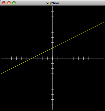
A first line: y=0.5x+2

Note on lists, arrays and matrices: You’ll notice that we create the curve, give it a list of x values (using arange), and then calculate the corresponding y values using matrix multiplication: 0.5 * line.x. This works because line.x actually stores the values as an an array, not as a list. The key difference between lists and arrays, as far as we’re concerned, is that we can get away with this type of multiplication with an array and not a list. However, an array is not a matrix, as is clearly demonstrated by the second part of the command where 2 is added to the result of the multiplication. In this case, 2 is added to each value in the array; if it were an actual matrix you need to add another matrix of the same shape that’s filled with 2’s. Right now, this is invisible to the students. The line of code makes sense. The concern is that when they do start working with matrices there might be some confusion. So watch out.

And to make any other function you just need to adjust the final line. So a parabola:
! y = x^2
would be:

line.y = line.x**2

(The two stars “**” indicates an exponent).

An Assignment

So, to assess learning, and to review the different functions we’ve learned, I asked students to produce “studies” of the different curves by demonstrating what happens when you change the different constants and coefficients in the equation.

For a straight line the general equation is:
! y = mx + b

you what happens when:

  • m > 1;
  • 0 < m < 1;
  • m < 0

and:

  • b > 1;
  • 0 < b < 1;
  • b < 0

The result is, after you add some labels, looks something like the image at the very top of this post.

This type of exercise can be done for polynomials, exponential, trigonometric, and almost any other type of functions.

How Long does it Take to Make a Vpython Program?

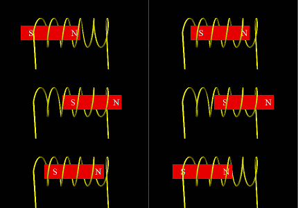
Moving the magnet through a wire coil creates an electric current in the wire. Animation captured from the VPython program: Magnetic Induction - Coils.

My students asked me this question the other day, and while slapping together an animation of electromagnetic induction I gave it some thought.

This program itself is really simple. It took about 15 minutes.

But that’s not counting the half hour I spent searching the web for an image I could use to illustrate magnetic induction and not finding one I could use.

Nor does it count the four hours I spent after I got the animation working to get the program to take screen captures automatically. Of course, I must admit that figuring out the screen captures would have gone a lot quicker if I’d not had to rebuild all my permissions on my hard drive (I’d recently reformatted it), and reinstall ImageMagick and gifsicle to take the screen captures and make animations.

Equations of a Parabola: Standard to Vertex Form and Back Again

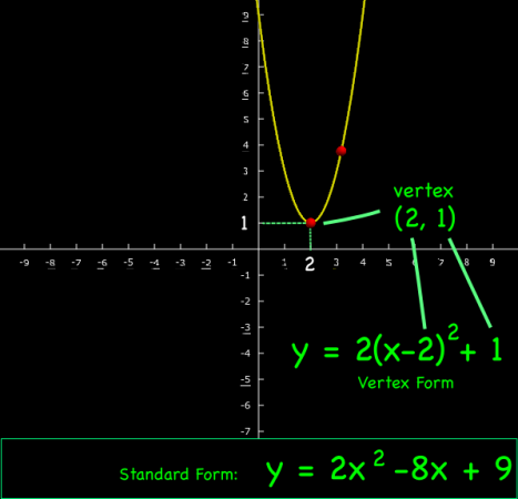
Highlighting the Vertex Form of the equation for a parabola.

The equation for a parabola is usually written as:

Standard form:
! y = ax^2 + bx + c

where a, b and c are constants. This is the form displayed in both the VPython Parabola and Excel parabola programs. However, to make the movement of the curve easier, the VPython program also uses the vertex form of the equation internally:

Vertex Form:
! y = a(x-h)^2 + k

where the point (h, k) is the location of the vertex of the parabola. In the example above, h = 1 and k = 2.

To translate between the two forms of the equation, you have to rewrite them. Start by expanding the vertex form:

y = a(x – h)2 + k

becomes:

y = a(x – h)(x – h) + k

multiplied out to get:

y = a(x2 – 2hx + h2) + k

now distribute the a:

y = ax2 – 2ahx + ah2 + k

finally, group all the coefficients:

y = (a)x2 – (2ah)x + (ah2 + k)

This equation has the same form as y = ax2 + bx + c if:

Vertex to Standard Form:

a = a
b = -2ah
c = ah2+k

And we can rearrange these equations to go the other way, to find the vertex form from the standard form:

Standard to Vertex Form:

! a = a
! h = \frac{\displaystyle -b}{\displaystyle 2a}
! k = c - ah^2 = c - \frac{\displaystyle b^2}{\displaystyle 4a}

Summary

In sum, you can write the standard equation for a parabola as:

Standard form:

And you can write the equation for the same parabola in vertex form as:

Vertex form:

UPDATES

UPDATE 1: This app will automatically convert from standard to vertex form (or back again).

UPDATE 2: Automatically generate and embed graphs using this parabolic grapher app.

Parabola Program

Animation showing the widening and shrinking of the parabola.

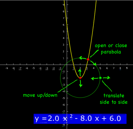
So I put together this interactive parabola program using VPython (code here) for students encountering these curves in Algebra.

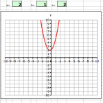
Simple Excel program to graph a parabola.

It’s a more interactive version of the Excel parabola program in that you can move the curve by dragging on some control points, rather than just having to enter the coefficients of the equation. The program is still in development, but it is at a useful stage right now, so I thought I’d make it available for anyone who wanted to try it.

The program is fairly straightforward to use. You can move the curve (translate it) up and down, and expand or tighten the area within the parabola.

The program also displays the equation of the curve in standard form:
! y = ax^2 + bx + c

.

What the buttons do.

Next Steps

I’m also working making the standard equation editable by clicking on it and typing, and am considering showing the x-axis intercepts, which will give algebra students a nice, visual way to of checking their factoring.

References

Coffman, J., 2011 (accessed). Translating Parabolas. http://www.jcoffman.com/Algebra2/ch5_3.htm

Math Warehouse, 2011 (accessed). Equation of a Parabola
Standard Form and Vertex Form Equations, http://www.mathwarehouse.com/geometry/parabola/standard-and-vertex-form.php#

WolframAlpha.com, 2011 (accessed). http://www.wolframalpha.com/input/?i=a^2+x^4%2Bx^2-r^2%3D0

Sling: A VPython Model Demonstrating Centripetal Force and Conservation of Angular Momentum

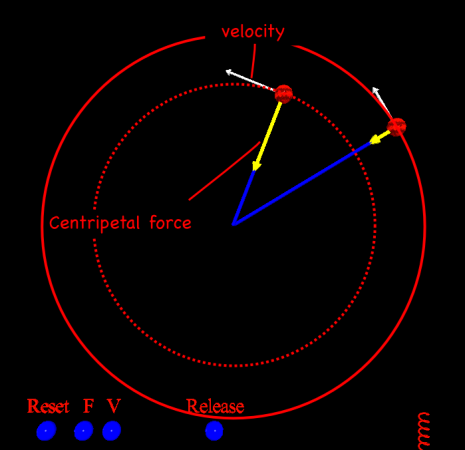
Animation captured from the sling.py Vpython model. The yellow arrow shows the centripetal force. The white arrow shows the velocity.

Sitting in a car that’s going around a sharp bend, its easy to feel like there’s a force pushing you against the side of the car. It’s called the centrifugal force, and while it’s real to you as you rotate with the car, if you look at things from the outside (from a frame of reference that’s not rotating) there’s really no force pushing you outward. The only force is the one keeping you in the car; the force of the side of the car on you. This is the centripetal force. Given all the potential for confusion, I created this little VPython model that mimics a sling.

Centripetal Force

In the model, you launch a ball and it goes off in a straight line. That’s inertia. An object will move in a straight line unless there’s some other force acting on it. When the ball hits the string, it catches and the string starts to pull on the ball, taking it away from its straight line trajectory. The force that pulls the ball away from its original straight path is the centripetal force.

Image from Stern (2004): (23a) Frames of Reference: The Centrifugal Force

Conservation of Angular Momentum

The ball rotating on the sling has an angular momentum (L) that’s equal to the velocity (v) times its mass (m) times its radius (r) away from the center.

L = mvr            , angular momentum

Now, angular momentum is conserved, which means that if you shorten the string, reducing the radius, something else must increase to compensate. Since the mass can’t change, the velocity has to, and the ball speeds up.

The ball on the string with the shorter radius has the higher velocity (moves faster). It also has a higher centripetal force. The ball for shortening the radius is not shown in this figure.

I’ve put in a little ball at the end of the string that you can pull on to shorten the radius.

Tangential Velocity

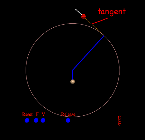
Once the ball is attached to the string, the centripetal force will keep it moving in a circle. If you release the ball then it will fly off in a straight line in whatever direction it was going when you released it. With no forces acting on the ball, inertia says the ball will move in a straight line.

The ball, when released from the string, flies off in a tangent.

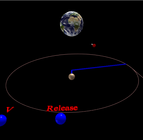
To better illustrate the ball’s motion off a tangent, I put in a target to aim for. It’s off the screen for the normal model view, but if you rotate the scene to look due north you’ll see it.