Projectile Motion

Abstract

A series of still photographs of a projectile (soccer ball) in motion were used to determine the equation for the height of the ball (h(t) = 4.9 t² + 14.2 t + 1.25), the initial velocity of the ball (14.2 m), the maximum height of the ball (11.6 m), and the time between each photograph (0.41 s). The problem was solved numerically using MS Excel’s Solver function. There are much easier ways of doing this, which we did not do.

Introduction

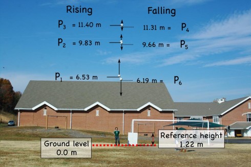
projectile-diagram — Figure 1. Calculated elevation of the soccer ball after launch.

projectile-3832c2-800 — Figure 2. Animation of the soccer ball projectile.

One of physics lab assignments I gave my students was to see if students could use a camera to capture a sequence of images of a projectile, plot the elevation of the projectile from the photographs, determine the constants in the parabolic equation for the height of the projectile, and, in so doing, determine the velocity at which the projectile was launched.

I offered my old, digital Pentax SLR that can take up to seven pictures in quick sequence and be set to fully manual. A digital video camera with a detailed timestamp would have been ideal, but we did not have one available at the time.

Now the easy way of getting the velocity data would be to estimate the heights (h) of the ball from the image using some sort of known reference (in this case the whiteboard), and determine the time between each photograph (Δt) by photographing a stopwatch using the same shutterspeed settings. After all, the average velocity of the ball between two images would be:

$! \bar{v} = \frac{\Delta h}{\Delta t}$

The reference whiteboard is four feet tall (1.22 m) in real life, but 51 pixels tall in the image. Using this ratio (i.e. 1.22 m = 51 px) we can convert the heights of the ball from pixels to meters:

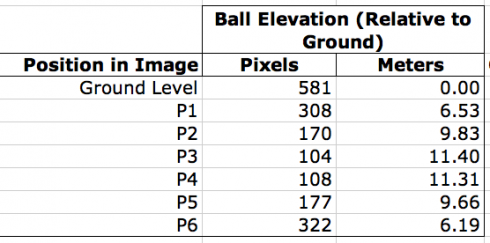
elevations — Table 1. Table showing the conversion of the height of the ball in pixels to elevation (in meters).

Unfortunately, I think my students forgot to do the pictures of the stopwatch to get Δt, the time between each photograph. Since the lab reports are due on Monday, and it’s the weekend now I’m curious to see what they come up with.

However, I was wondering if they could use just the elevation data to back out the Δt. So I gave it a try myself. Even the easiest way of solving this problem is not trivial, in fact, I ended up resorting to Excel’s iterative solver to find the answers. While this procedure probably goes a little beyond what I expect from the typical high school physics student, more advanced students who are taking calculus might benefit.

Procedure

We took the reference whiteboard (1.21 m tall), a soccer ball, and the camera outside. The whiteboard was leant vertically against the post of the soccer goal. The ball was thrown vertically by a student standing next to the whiteboard (see Figure 1) while pictures were taken. The camera’s shutterspeed was 1/250th of a second. The distance from the camera to the person throwing the ball (and to the whiteboard) were not measured.

The procedure was repeated several times, but only one trail was used in this analysis.

The images were loaded onto a computer, and the program GIMP was used to determine the distance, in pixels, from the ground to the projectile. The size of the reference whiteboard, in pixels, was used to calculate the height of the soccer ball in meters.

The elevations measured off the photographs were then used to calculate the release velocity, time between snapshots, and maximum height of the ball.

The Equation for Elevation

I started with the fact that once the ball is released, the only force acting on it is the force of gravity. Since the mass of the ball does not change we only have to consider the acceleration due to gravity (-9.8 m/s²). I also neglect air resistance to make things easier.

Finding the Velocity Equation

Start with the fact that, acceleration is the rate of change of velocity with time. You can write it in the differential form:

$! a = \frac{dv}{dt} = -9.8$

so we integrate with respect to time to get the equation for velocity as a function of time:

$! v(t) = \int -9.8 dt$

$! v(t) = -9.8 t + c$

where c is an unknown constant. What we do know though, is that at the beginning, when the ball is just launched, time is zero (t = 0) so c_v becomes the initial velocity (v₀) at which the ball is thrown:

at t = 0, v(0) = v₀:
$! v_0 = -9.8 (0) + c$

$! v_0 = c$

So our velocity equation becomes:

$! v(t) = -9.8 t + v_0$

Finding the height equation

Now since we know that velocity is the rate of change of distance (in this case height) with time:

$! v(t) = \frac{dh}{dt} = -9.8 t + v_0$

so we integrate again to find the height equation:

$! \frac{dh}{dt} = -9.8 t + v_0$
$! h(t) = \int (-9.8 t + v_0) dt$
$! h(t) = \frac{-9.8 t^2}{2} + v_0 t + c$

Similar to what we did with the velocity equation, to find the new constant c we consider what happens at the start time, when the ball is launched, and t = 0 and h(0) = h₀;

$! h_0 = \frac{-9.8 (0)^2}{2} + v_0 (0) + c$

so:
$! h_0 = c$

The constant is equal to the initial height of the ball — the height of the ball when it’s thrown. So we end up with the final equation:

$! h(t) = \frac{-9.8 t^2}{2} + v_0 t + h_0$

Results

Solving all the unknowns

At this point, although we have an equation for the height of the ball, we don’t know the initial velocity (v₀), nor do we know the initial height of the ball when it’s released (h₀). And we still don’t know the time when the ball is at each position.

With that many unknowns we’d need the same number of independent equations to be able to solve for them all. It may be possible, but instead of analytically solving the equations I opted to take a numerical approach, and use Excel’s Solver function.

I started by setting up the equations to calculate the height of the ball at six different times to correspond with our six height measurements. It was necessary therefore to create a set of variables:

Time when we started taking pictures (t₁): Since we don’t know how long after we threw the ball we started taking pictures, I made this a variable called t₁.
The time between each picture (dt): I made the assumption that the time between each picture would be constant. The shutter speed was constant (1/250th of a second) so there is no obvious reason why the time should be different.
Initial velocity (v₀): The initial upward speed at which the ball was thrown. Obviously, the faster the initial speed the higher the ball goes, so this is a fairly important parameter.
Initial height (h₀): We also don’t precisely know how high the ball was when it was released, so this also needs to be a variable.

By defining the time between each picture as dt, we can write the time that each picture was taken in terms of the time of the initial picture (t₁) and dt. After all the second picture would have been taken dt seconds after the first for a total time of:

$! t(P2) = t_0 + dt$

similarly for all the pictures:

photo-times — Table 2. Table of expressions giving the time when each of the six photos were taken.

Now I set up an Excel spreadsheet and gave all the unknown variable values and initial value of 1:

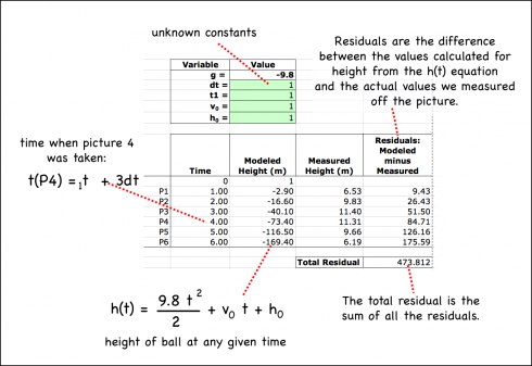
excel-solver — Table 3. Table in Excel for determining the height of a projectile. All of the unknown variables' values are highlighted in green and have been given an initial value of 1.

Now I just had to run Solver and tell it that I wanted the Total Residual, which gives the difference between the h(1) equation’s values for height and the actual, measured values, to be as close to zero as possible. A perfect fit of the equation to the data would have a total residual of one, but that’s not possible when you’re dealing with real data.

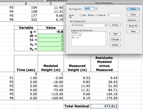
solving — Table 4. Parameters set in Solver to determine the values of the unknown constants.

Even so, I had to goose Solver a bit for it to produce reasonable numbers. I put in a few constraints:

dt >= 0: We could not have a negative time between pictures.
h₀ <= 1.25: 1.25 meters seemed reasonable for the height at which the ball was released.
t₁ <= 1: It also seemed reasonable that the time when the first picture was taken was less than one second after the ball was thrown.

I ran the Solver a few times, and had to reset dt to 0.5 at one point when it had become zero, but the final result looked remarkably good: the total difference between the modeled line and the actual data was only 0.113 meters.

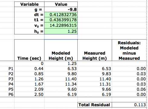
solver-after — Table 5. Solver's solution for the unknown constants in the height equation.

So we found that:

Initial velocity: v₀ = 14.2 m/s
Height at release: h₀ = 1.25 m
Time between pictures: dt = 0.41 s
Time when the first picture was taken: t₁ = 0.44 s

Which makes the height equation:

$! h(t) = \frac{-9.8 t^2}{2} + 14.2 t + 1.25$

Using these constants in the height equation, we could see how good fit the height equation was to the data:

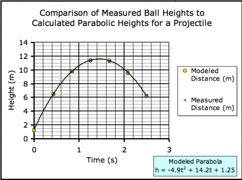
projectile-graph — Figure 3. Graph comparing the modeled heights (from the h(t) equation) to the actual data.

Maximum Height of the Ball

Finally, the maximum height of the ball can be read off the graph, but it can also be determined using the equation for the height of the ball:

$! h(t) = \frac{-9.8 t^2}{2} + v_0 t + h_0$

We know that the maximum height is reached when the ball stops moving upward and starts to descend. At that point, the vertical velocity of the ball is zero. Since the velocity of the ball is the rate of change of height ( $v = \frac{dh}{dt}$ ) we can differentiate the height equation to get an equation for velocity.

$! h(t) = \frac{-9.8 t^2}{2} + v_0 t + h_0$

$! v = \frac{dh}{dt} = -9.8 t + v_0$

since we’ve determined that the initial velocity of the ball is 14.2 m/s we get:

$! v = -9.8 t + 14.2$

when the velocity is zero (v = 0):

$! 0 = -9.8 t + 14.2$

which can be solved for t to find that the time the ball reaches it’s maximum height is:

$! t = 1.45 seconds$

Putting this into the height equation:

$! h(1.45) = \frac{-9.8 (1.45)^2}{2} + 14.2 (1.45) + 1.25$

gives:

$! h_{max} = 11.58 meters$

Discussion

I’m quite happy with the way this project turned out. The fit between the modeled heights (h(t)) and the actual heights was very good.

My primary concern going into the project was that the distortion from the camera lens would make this technique impossible, but that appears not to be a significant problem.

Most of this calculation, including the somewhat tricky numerical solution using Solver could have been avoided if I’d calibrated the camera, simply by pointing it at a stopwatch (using the same shutterspeed as in the experiment) and measuring the time between snapshots. It will therefore be interesting to see if the actual time between shots (dt) is close to the dt of 0.41 seconds calculated by the model.

Finally, as noted above, a video camera with a timestamp would possibly be a more useful technology for this experiment.

Conclusion

It is possible to analyze the projectile path of an object using a series of snapshots, to determine the initial velocity of the projectile, its release height, and the time between snapshots, if you can assume that the time between snapshots is identical. There are, however, much easier methods of solving this problem.

References

None, but this is where they’d be if I had any.

Appendix

The Excel spreadsheet where all the calculations were done is here.

Morning Fog

lake-am-3815c2 — Early morning fog over the lake.

There’s a place on the road to school where you crest a little rise and the St. Albans golf course opens up before you. “Zen-like,” I’ve heard it described. On one lovely fall morning last week the view was absolutely ridiculous. I had to stop.

Resisting the coming winter, warmer air from down south just pushed over the hills overnight, trapping the cooler air in the valley, creating a thermal inversion that trapped a layer of fog just below the tops of the hills. Small tendrils of mist were rising off lake in the bottom of the valley, feeding the fog layer as the cooler valley air condensed the water vapor evaporating off the still warm lake.

Combine the fog, mists, early morning sunlight just beginning to reach into the valley, and the brilliant fall colors contrasting against the still-green lawns, and the result was absolutely amazing.

lake-am-b-300 — Not being able to leave well enough alone, I've also put together this "3d" gif. It does show the fog on the lake nicely though.

Figuring Out Experimental Error

Using stopwatches, we measured the time it took for the tennis ball to fall 5.3 meters. Some of the individual measurements were off by over 30%, but the average time measured was only off by 7%.

I did a little exercise at the start of my high-school physics class today that introduced different types of experimental error. We’re starting the second quarter now and it’s time for their lab reports to including more discussion about potential sources of error, how they might fix some of them, and what they might mean.

One of the stairwells just outside the physics classroom wraps around nicely, so students could stand on the steps and, using stopwatches, time it as I dropped a tennis ball 5.3 meters, from the top banister to the floor below.

measured-falling-time — Students' measured falling times (in seconds).

Random and Reading Errors

They had a variety of stopwatches, including a number of phones, at least one wristwatch, and a few of the classroom stopwatches that I had on hand. Some devices could do readings to one hundredth of a second, while others could only do tenths of a second. So you can see that there is some error just due to how detailed the measuring device can be read. We’ll call this the reading error. If the best value your stopwatch gives you is to the tenth of a second, then you have a reading error of plus or minus 0.1 seconds (±0.1 s). And you can’t do much about this other than get a better measuring device.

Another source of error is just due to random differences that will happen with every experimental trial. Maybe you were just a fraction of a second slower stopping your watch this time compared to the last. Maybe a slight gust of air slowed the balls fall when it dropped this time. This type of error is usually just called random error, and can only be reduced by taking more and more measurements.

Our combination of reading and random errors, meant that we had quite a wide range of results – ranging from a minimum time of 0.7 seconds, to a maximum of 1.2 seconds.

So what was the right answer?

Well, you can calculate the falling time if you know the distance (d) the ball fell (d = 5.3 m), and its acceleration due to gravity (g = 9.8 m/s²) using the equation:

$! t = \sqrt{\frac{2d}{g}}$

which gives:

$! t = 1.043 s$

So while some individual measurements were off by over 30%, the average value was off by only 8%, which is a nice illustration of the phenomenon that the more measurements you take, the better your result. In fact, you can plot the improvement in the data by drawing a graph of how the average of the measurements improves with the number of measurements (n) you take.

falling-averages — The first measurement (1.2 s) is much higher than the calculated value, but when you incorporate the next four values in the average it undershoots the actual (calculated) value. However, as you add more and more data points into the average the measured value gets slowly closer to the calculated value.

More measurements reduce the random error, but you tend to get to a point of diminishing returns when you average just does not improve enough to make it worth the effort of taking more measurements. The graph shows the average slowly ramping up after you use five measurements. While there are statistical techniques that can help you determine how many samples are enough, you ultimately have to base you decision on how accurate you want to be and how much time and energy you want to spend on the project. Given the large range of values we have in this example, I would not want to use less than six measurements.

Systematic Error

But, as you can see from the graph, even with over a dozen measurements, the average measured value remains persistently lower than the calculated value. Why?

This is quite likely due to some systematic error in our experiment – an error you make every time you do the experiment. Systematic errors are the most interesting type of errors because they tell you that something in the way you’ve designed your experiment is faulty.

The most exciting type of systematic error would, in my opinion, be one caused by a fundamental error in your assumptions, because they challenge you to fundamentally reevaluate what you’re doing. The scientists who recently reported seeing particles moving faster than light made their discovery because there was a systematic error in their measurements – an error that may result in the rewriting of the laws of physics.

In our experiment, I calculated the time the tennis ball took to fall using the gravitational acceleration at the surface of the Earth (9.8 m/s²). One important force that I did not consider in the calculation was air resistance. Air resistance would slow down the ball every single time it was dropped. It would be a systematic error. In fact, we could use the error that shows up to actually calculate the force of the air resistance.

However, since air resistance would slow the ball down, it would take longer to hit the floor. Unfortunately, our measurements were shorter than the calculated falling time so air resistance is unlikely to explain our error. So we’re left with some error in how the experiment was done. And quite frankly, I’m not really sure what it is. I suspect it has to do with student’s reaction times – it probably took them longer to start their stopwatches when I dropped the ball than it did to stop them when the ball hit the floor – but I’m not sure. We’ll need further experiments to figure this one out.

In Conclusion

On reflection, I think I probably would have done better using a less dense ball, perhaps a styrofoam ball, that would be more affected by air resistance, so I can show how systematic errors can be useful.

Fortunately (sort of) in my demonstration I made an error in calculating the falling rate – I forgot to include the 2 under the square root sign – so I ended up with a much lower predicted falling time for the ball – which allowed me to go through a whole exercise showing the class how to use Excel’s Goal Seek function to figure out the deceleration due to air resistance.

My Excel Spreadsheet with all the data and calculations is included here.

There are quite a number of other things that I did not get into since I was trying to keep this exercise short (less than half an hour), but one key one would be using significant figures.

There are a number of good, but technical websites dealing with error analysis including this, this and this.