How the Immune System Works

Awesome video by Kurzgesagt explaining “Why You Are Still Alive“.

Art, Science and Math

The Tabletop Whale blog by Elanor Lutz, has a focus on scientific illustration. It is a wonderful intersection of science, math and art, such as in this beautiful animation of a muscle in motion.

She has animations of butterflies and birds in motion as well.

Perhaps not surprisingly, my middle school students have a difficult time wrapping their heads around the idea of multiple frames of reference. We were in a canoe on the Current River and I asked the student paddling in the rear of the boat to look at me and answer the question, “Are we in the canoe moving, or are we steady in one spot and everything around us moving?”

This resulted in some serious cognitive processing. And she still has not gotten back to me with an answer.

Another student, faced with the same question, thought it over overnight and concluded that it was a riddle. He figured the correct answer was that the canoe was moving and the land was still. I asked him to think about it a little more (because he was only half right).

Interestingly enough, I’ll be teaching my Advanced Physics class this block, and the first chapter has a neat little section on coordinate systems. I’m curious to see if the 11th and 12th graders have an easier time with the concept.

Finnish Education

A documentary on the educational system in Finland which is ranked as one of the best in the world. They have little homework, no standardized testing, and are rather Montessori-like.

Parts 2, 3, and 4.

Updated Atom Builder

A couple of my students asked for worksheets to practice drawing atoms and electron shells. I updated the Atom Builder app to make sure it works and to make the app embedable.

So now I can ask a student to draw ²³Na⁺ then show the what they should get:

Worksheet

Draw diagrams of the following atoms, showing the number of neutrons, protons, and electrons in shells. See the example above.

¹⁴C: answer.
³²K⁺: answer.
¹⁸O^2-: answer.
⁴He²⁺: answer.
³²P^–: answer.

I guess the next step is to adapt the app so you can hide the element symbol so student have to figure what element based on the diagram.

Math Gifs

Mike Schmidt passed along this link to Lisa Winter’s post collecting 21 GIFs That Explain Mathematical Concepts.

For example:

Converting a trigonometric function (sin curve) from Cartesian to polar coordinates. Source: “Cartesian to polar” by Kieff – Own work. Licensed under Public domain via Wikimedia Commons.

Differentiation Using Limits

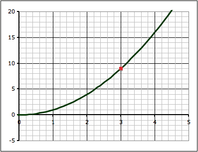
We can use the idea of limits to come up with some general relationships between functions and their slopes. Take, for example, the last project where we found the slope of the function y = x² at the point where x = 3:

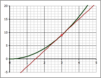
The green line is the curve y = x2 and the straight red line is the tangent to the curve at the point where x = 3 (i.e. at (3,9)). — The green line is the curve *y = x²* and the straight red line is the tangent to the curve at the point where *x = 3* (i.e. at (3,9)).

Finding the approximate slope using a forward difference.

We found the slope of the tangent line at the point (3,9) by a series of approximations. First we took two points on the curve, (3,9) and (4,16) and found the slope between those two points.

The equation for slope can be written in any of these three ways:

we find the exact slope by taking points on the line closer and closer together (which means that Δx is getting smaller and smaller). In math-speak, we’re saying that we’re taking the limit of the slope equation as Δx approaches zero.

Since we’re taking Δx to zero we might as well ask what happens to the slope when Δx is equal to zero.

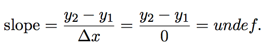
As we can see from the equation, we end up with zero on the denominator, which makes the whole thing undefined, which we really do not want.

But what if we can rearrange things to get the Δx out of the denominator?

Let’s rewrite the equation y = x² as a function:

$f(x) = x^2$

So the point we’re interested in find the slope at is just (x, f(x)), which in this case happens to be (3, 9), but we’re not going to be using the actual numbers anymore so we can come up with a more general relationship.

To find the slope we find the point where the value on the x-axis is x and the value on the y-axis is f(x). — To find the slope we find the point where the value on the x-axis is x and the value on the y-axis is *f(x)*.

Now, and this is often the tricky part, the second point we use is going to have an x value of x + Δx:

For the second point, the x value we use is the first x offset by Δx.

which means that the value on the curve is f(x+Δx):

Our second point is where the x value is x+Δx and the y value is f(x+Δx). — Our second point is where the x value is *x+Δx* and the y value is *f(x+Δx)*.

So lets carefully observe the notation here. To find the slope of a line we can use the equation:

But with the function notation:

y₁ = f(x)
y₂ = f(x+Δx)

so:

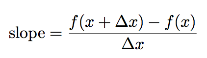
Now watch very carefully as I replace the function notation with the actual functions, specifically:

f(x) = x²
f(x+Δx) = (x+Δx)²

to give:

and if you understand how this, we’re almost all there, because the rest is algebra.

We simplify the equation above by expanding the numerator.

now we can subtract the similar terms (x²) and divide through by Δx to get:

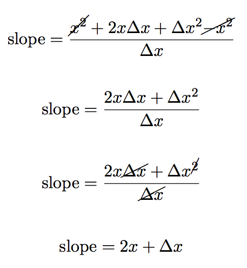
But remember we don’t just want the slope, we want to find the slope where Δx approaches zero:

The problem before was that if we made Δx = 0 the equation would be undefined. But now, however, as Δx = 0 the second term in the equation just goes to zero:

leaving us just with the first term 2x:

Remember that we were trying to do this at the point where x = 3. So if we put x = 3 into this equation we get:

Which we know is the right answer because we did the very problem by hand already.

but now however we’ve come up with a more general equation for the slope. With it we can easily find the slope of our curve at any point along the curve!

For example, what is the slope of the curve when x = 0:

Notation

Now it’s a bit cumbersome to write the limit as Δx goes to zero every time, so we’ll instead call our equation for the slope of the line the differential, and we’ll give it the notation as the function prime:

i.e. if we have a function f(x) = x²:

we write its differential as:

To confuse things (at least for the moment) there are a number of ways of writing the differential (the different methods are useful in different contexts), so you will see things like:

So now that we know how to find the differential using limits, we’ll practice finding the differential of polynomial functions and see if we can find a general pattern that allows us to bypass the whole limits thing altogether.

Finding the Limit (Following up the Guitar Project)

Following up on the project to find the volume (and surface area) of a guitar, and the slope at a point along the outline of the guitar, I asked students to use the same techniques to estimate the area under a curve (y = x²) and find the slope at a point along the curve. Specifically:

Draw the function y = x²
Find the area bounded by the function, the lines x = 1 and x = 4, and the x-axis
Find the slope of a tangent to the y = x² function at the point where x = 3.

The point of the second question is to test if students have internalized the idea that they can approximate curved shapes with trapezoids, but they have to weigh the time it will take to do a lot of trapezoids, versus the reduction in error that will result from more trapezoids. It’s interesting to see students’ character come through in this assignment: some choose to make one big trapezoid and are done, while other will go so many trapezoids that they run out of time to get them done.

It just occurs to me, however, that an interesting way to assess this assignment would be to give them a fixed time, and tell them that their score will be the 100 minus the percent error in their calculations.

Limits

The third question–about finding the slope of a tangent line at x = 3–is our jumping off point into the mathematics of limits and calculus.

Some students do a single approximation–either forward or backward–, while others do both and take the average.

The forward approximation involves finding the values for the function y = x² at x = 3 and x = 4 and finding the slope between the two points:

when x = 3, y = 9, so we have the point (x₁,y₁) = (3, 9)
when x = 4, y = 16, so we have the point (x₂,y₂) = (3, 16)

The slope (m) between two points is found with the equation they learned back in algebra:

$\text{slope} = m = \frac{\Delta y}{\Delta x} = \frac{y_2-y_1}{x_2-x_1} = \frac{y_2-y_1}{\Delta x}$

Where Δx = x₂-x₁ and Δy = y₂-y₁.

Using the two points above gives:

$\text{slope} = m = \frac{\Delta y}{\Delta x} = \frac{16-9}{4-3} = \frac{7}{1} = 7$

Those who use the backward approximation simply use the point when x = 2 instead of x = 4, and they end up with a value for the slope of 5.

Averaging the forward and backward approximations give a slope of 6.

Now, since they know that the closer you make the points the better the approximation, I ask them to make a table to see what happens as they do so. This means reducing the value of Δx. In both the forward and backward approximation shown above, Δx = 1.

This can be done very quickly in Excel (or any other spreadsheet program), however, this time at least, most students chose to do it by hand. They end up with a table that looks like this:

As dx gets smaller the calculated slope approaches 6.

As the difference in x gets smaller and approaches zero, the slope approaches 6.

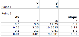
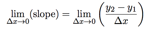
As you plot slope versus the change in x (Δx), you can see that as Δx gets smaller and smaller and approaches zero, the slope gets closer and closer to 6. So we could say that:

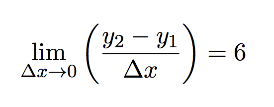
the limit of the slope as Δx approaches zero is 6.

Mathematically this can be written as:

or using the equation for slope:

Now, we can work on taking the limit in a more general way to do differentiation.

Year: 2014