The Math of Music

Mark French has an excellent YouTube channel on Mechanical Engineering, including the above video on Math and Music. The video describes the mathematical relationships between musical notes.

Given the sequence of notes: C, C#, D, D#, E, F, F#, G, G#, A, A#, B, C.

Let the frequency of the C note be f0, the frequency of C# be f1 etc.

The ratio of any two successive frequencies is constant (r). For example:

 \frac{f_1}{f_0} = r

so:

 \frac{f_1}{f_0} = \frac{f_2}{f_1} = \frac{f_4}{f_3} = \frac{f_{12}}{f_{11}} = r

We can find the ratio of the first and third notes by combining the first two ratios. First solve for f1 in the first equation:

 \frac{f_1}{f_0} = r

solving for f1,

 f_1 = f_0 \; r

now take the second ratio:

 \frac{f_2}{f_1} = r

and substitute for f1,

 \frac{f_2}{f_0 \; r} = r

which gives:

 \frac{f_2}{f_0} = r^2

We can now generalize to get the formula:

 \frac{f_n}{f_0} = r^n

or

 f_n = f_0 \; r^n

where,

  • n – is the number of the note

From this we can see that comparing the ratio of the first and last notes (f12/f0) is:

 \frac{f_{12}}{f_0} = r^{12}

Now, as we’ve seen before, when we talked about octaves, the frequency of the same note in two different octaves is a factor of two times the lower octave note.
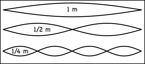
Click the waves to hear the different octaves. The wavelengths of the sounds are shown (in meters).


So, the frequency ratio between the first C (f0) and the second C (f12) is 2:

 \frac{f_{12}}{f_0} = 2

therefore:

 \frac{f_{12}}{f_0} = 2 = r^{12}

so we can now find r:

 r^{12} = 2

 r = \sqrt[12]{2}

Finally, we can now find the frequency of all the notes if we know that the international standard for the note A4 is 440 Hz.

Mark French has details on the math in his two books: Engineering the Guitar which is algebra based, and Technology of the Guitar, which is calculus based.

Waves in the Creek

Waves in the creek.
Waves in the creek.

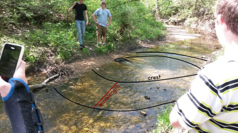
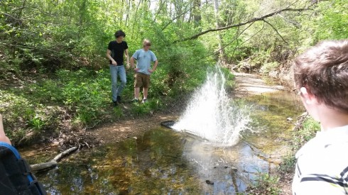
We talked about waves today down at the creek. The water was fairly calm so we could make some nice surface waves using floating leaves to show the up-down/side-to-side motion as the waves passed. I gave them 10 minutes to “play”, and more than one team tried to make a tsunami.

Creating a large wave.

Since it’s allergy season, one student who could not go outside, read the chapter on the characteristics of waves and prepared a short–5 minutes–presentation for the rest of the class when we came back in.

Annotated image highlighting the crests of the waves and the wavelength.

Radiolab: The Extinction of the Dinosaurs

RadioLab has an excellent podcast featuring Jay Melosh, a geophysicist who specializes in impact craters, and who advocates the hypothesis that the entire extinction event that killed off the dinosaurs at the boundary between the Cretaceous and Tertiary (the K-T boundary) took place over a period of two hours. The asteroid impact vaporized the crust of the Earth where it hit (near the Yucatan peninsula) and blasted this rock gas into space. There it cooled down to create little glass particles that reentered the atmosphere. On reentry the glass burned up, but there was so much of it that it raised the temperature of the atmosphere by several hundred degrees Celsius. Anything near the surface (mostly the dinosaurs) was cooked, but anything living just beneath the surface could have survived.

Electricity and Magnetism Experiments

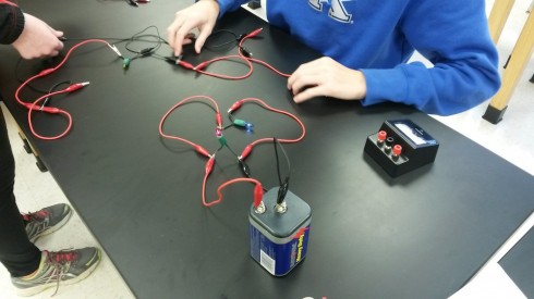
Building bulbs into parallel circuits.

Last week, my middle schoolers did a set of experiments on electricity and magnetism. They answered the questions:

  • How does the voltage across each light bulb change as you add more and more bulbs to a parallel circuit?
  • How does the voltage across each light bulb change as you add more and more bulbs to a series circuit?
  • How does the number of coils of wire wrapped around a nail affect it’s magnetism (as measured by the number of paperclips it can pick up)?
  • How does the amount of salt mixed into water affect its conductivity?
An electromagnetic nail lifts two paperclips.
Students measure the conductivity of a salt water solution.

Each question is designed so that students have something to measure and will be able to use those measurements to make predictions. For example, once they’ve measured the voltage across four bulbs in series, they should be able to predict the voltage across the bulbs in a series of ten.

Some of the experiments, like the nail electromagnet, should have simple linear trends, with students choosing the advanced option having to find an equation to fit their data for the predictions. And I’ll challenge the students in Algebra II to find the equations for the inverse relationships–I’ve already asked their math teacher (Mr. Schmidt) to help them out if they need it.

This has also provided the opportunity for them to apply what they’ve just learned about drawing circuit diagrams (we use this set of symbols).

Circuit diagrams of bulbs in parallel. The voltage difference across each bulb is also noted.

Parabolic Trajectories

The post below was contributed by Michael Schmidt, our math teacher.

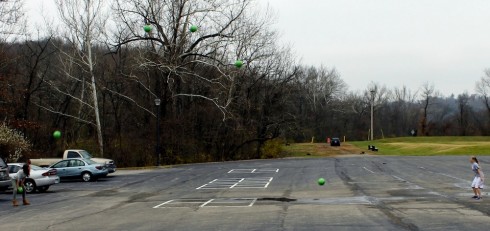
Layered image showing the ballistic path of the green ball thrown by two middle school students. Image by Michael Schmidt.

Parabolas can be a daunting new subject for some students. Often students are not aware of why a parabola may be useful. Luckily, nature always has an answer. Most children realize that a ball thrown through the air will fallow a particular arch but few have made the connected this arch to a parabola. Wonderfully, with a little technology this connection can be made.

With Ms. Hahn’s Canon SLR, I had some of my students throw a ball around outside and took a series of quick pictures of the ball in flight. Since my hand is not very steady, I took the pictures and used the Hugin’s image_stack_align program to align each photo so I could stack them in GIMP.

Within GIMP, I layered the photos on top of each other and cut out the ball from each layer then composed those onto one image. Careful not to move the ball since our later analysis will be less accurate. The result will look something like the following:

Now that there is an image for student to see, we can determine the ball’s height at each point using their own height as a reference. We can then use this information to model a parabola to the data with a site like: http://www.arachnoid.com/polysolve/ .

For the more advanced student an investigation of the least-squares algorithm used by the site may be done.

Now, once we have an expression for the parabola, students can compare how fast they sent the ball into the air.