Programming – Page 4 – Montessori Muddle

Sorting algorithms (with Hungarian Dance)

This TedEd video explains a few common sorting methods used in computer science. Sorting can be a challenging computational problem because of the enormous number of comparisons between items that can be involved, so computer scientists has spent a lot of time looking into it.

The video below shows the Quick Sort method using Hungarian folk dance.

Numerical and Analytical Solutions 2: Constant Acceleration

Previously, I showed how to solve a simple problem of motion at a constant velocity analytically and numerically. Because of the nature of the problem both solutions gave the same result. Now we’ll try a constant acceleration problem which should highlight some of the key differences between the two approaches, particularly the tradeoffs you must make when using numerical approaches.

The Problem

A ball starts at the origin and moves horizontally with an acceleration of 0.2 m/s². Print out a table of the ball’s position (in x) with time (every second) for the first 20 seconds.

Analytical Solution
We know that acceleration (a) is the change in velocity with time (t):

$a = \frac{dv}{dt}$

so if we integrate acceleration we can find the velocity. Then, as we saw before, velocity (v) is the change in position with time:

$v = \frac{dx}{dt}$

which can be integrated to find the position (x) as a function of time.

So, to summarize, to find position as a function of time given only an acceleration, we need to integrate twice: first to get velocity then to get x.

For this problem where the acceleration is a constant 0.2 m/s² we start with acceleration:

$\frac{dv}{dt} = 0.2$

which integrates to give the general solution,

$v = 0.2 t + c$

To find the constant of integration we refer to the original question which does not say anything about velocity, so we assume that the initial velocity was 0: i.e.:

at t = 0 we have v = 0;

which we can substitute into the velocity equation to find that, for this problem, c is zero:

$v = 0.2 t + c$
$0 = 0.2 (0) + c$
$0 = c$

making the specific velocity equation:
$v = 0.2 t$

we replace v with dx/dt and integrate:

$\frac{dx}{dt} = 0.2 t$
$x = \frac{0.2 t^2}{2} + c$
$x = 0.1 t^2 + c$

This constant of integration can be found since we know that the ball starts at the origin so

at t = 0 we have x = 0, so;

$x = 0.1 t^2 + c$
$0 = 0.1 (0)^2 + c$
$0 = c$

Therefore our final equation for x is:

$x = 0.1 t^2$

Summarizing the Analytical

To summarize the analytical solution:

$a = 0.2$
$v = 0.2 t$
$x = 0.1 t^2$

These are all a function of time so it might be more proper to write them as:

$a(t) = 0.2$
$v(t) = 0.2 t$
$x(t) = 0.1 t^2$

Velocity and acceleration represent rates of change which so we could also write these equations as:

$a(t) = \frac{dv}{dt} = 0.2$
$v(t) = \frac{dx}{dt} = 0.2 t$
$x(t) = x = 0.1 t^2$

or we could even write acceleration as the second differential of the position:

$a(t) = \frac{d^2x}{dt^2} = 0.2$
$v(t) = \frac{dx}{dt} = 0.2 t$
$x(t) = x = 0.1 t^2$

or, if we preferred, we could even write it in prime notation for the differentials:

$a(t) = x''(t) = 0.2$
$v(t) = x'(t) = 0.2 t$
$x(t) = x(t) =0.1 t^2$

The Numerical Solution

As we saw before we can determine the position of a moving object if we know its old position (x_old) and how much that position has changed (dx).

$x_{new} = x_{old} + dx$

where the change in position is determined from the fact that velocity (v) is the change in position with time (dx/dt):

$v = \frac{dx}{dt}$

which rearranges to:

$dx = v dt$

So to find the new position of an object across a timestep we need two equations:

$dx = v dt$
$x_{new} = x_{old} + dx$

In this problem we don’t yet have the velocity because it changes with time, but we could use the exact same logic to find velocity since acceleration (a) is the change in velocity with time (dv/dt):

$a = \frac{dv}{dt}$

which rearranges to:

$dv = a dt$

and knowing the change in velocity (dv) we can find the velocity using:

$v_{new} = v_{old} + dv$

Therefore, we have four equations to find the position of an accelerating object (note that in the third equation I’ve replaced v with v_new which is calculated in the second equation):

$dv = a dt$
$v_{new} = v_{old} + dv$
$dx = v_{new} dt$
$x_{new} = x_{old} + dx$

These we can plug into a python program just so:

motion-01-both.py

from visual import *

# Initialize
x = 0.0
v = 0.0
a = 0.2
dt = 1.0

# Time loop
for t in arange(dt, 20+dt, dt):

     # Analytical solution
     x_a = 0.1 * t**2

     # Numerical solution
     dv = a * dt
     v = v + dv
     dx = v * dt
     x = x + dx

     # Output
     print t, x_a, x

which give output of:

>>> 
1.0 0.1 0.2
2.0 0.4 0.6
3.0 0.9 1.2
4.0 1.6 2.0
5.0 2.5 3.0
6.0 3.6 4.2
7.0 4.9 5.6
8.0 6.4 7.2
9.0 8.1 9.0
10.0 10.0 11.0
11.0 12.1 13.2
12.0 14.4 15.6
13.0 16.9 18.2
14.0 19.6 21.0
15.0 22.5 24.0
16.0 25.6 27.2
17.0 28.9 30.6
18.0 32.4 34.2
19.0 36.1 38.0
20.0 40.0 42.0

Here, unlike the case with constant velocity, the two methods give slightly different results. The analytical solution is the correct one, so we’ll use it for reference. The numerical solution is off because it does not fully account for the continuous nature of the acceleration: we update the velocity ever timestep (every 1 second), so the velocity changes in chunks.

To get a better result we can reduce the timestep. Using dt = 0.1 gives final results of:

18.8 35.344 35.532
18.9 35.721 35.91
19.0 36.1 36.29
19.1 36.481 36.672
19.2 36.864 37.056
19.3 37.249 37.442
19.4 37.636 37.83
19.5 38.025 38.22
19.6 38.416 38.612
19.7 38.809 39.006
19.8 39.204 39.402
19.9 39.601 39.8
20.0 40.0 40.2

which is much closer, but requires a bit more runtime on the computer. And this is the key tradeoff with numerical solutions: greater accuracy requires smaller timesteps which results in longer runtimes on the computer.

Post Script

To generate a graph of the data use the code:

from visual import *
from visual.graph import *

# Initialize
x = 0.0
v = 0.0
a = 0.2
dt = 1.0

analyticCurve = gcurve(color=color.red)
numericCurve = gcurve(color=color.yellow)
# Time loop
for t in arange(dt, 20+dt, dt):

     # Analytical solution
     x_a = 0.1 * t**2

     # Numerical solution
     dv = a * dt
     v = v + dv
     dx = v * dt
     x = x + dx

     # Output
     print t, x_a, x
     analyticCurve.plot(pos=(t, x_a))
     numericCurve.plot(pos=(t,x))

which gives:

Comparison of numerical and analytical solutions using a timestep (dt) of 1.0 seconds.

Numerical versus Analytical Solutions

We’ve started working on the physics of motion in my programming class, and really it boils down to solving differential equations using numerical methods. Since the class has a calculus co-requisite I thought a good way to approach teaching this would be to first have the solve the basic equations for motion (velocity and acceleration) analytically–using calculus–before we took the numerical approach.

Constant velocity

Question 1. A ball starts at the origin and moves horizontally at a speed of 0.5 m/s. Print out a table of the ball’s position (in x) with time (t) (every second) for the first 20 seconds.

Analytical Solution:
Well, we know that speed is the change in position (in the x direction in this case) with time, so a constant velocity of 0.5 m/s can be written as the differential equation:

$\frac{dx}{dt} = 0.5$

To get the ball’s position at a given time we need to integrate this differential equation. It turns out that my calculus students had not gotten to integration yet. So I gave them the 5 minute version, which they were able to pick up pretty quickly since integration’s just the reverse of differentiation, and we were able to move on.

Integrating gives:

$x = 0.5t + c$

which includes a constant of integration (c). This is the general solution to the differential equation. It’s called the general solution because we still can’t use it since we don’t know what c is. We need to find the specific solution for this particular problem.

In order to find c we need to know the actual position of the ball is at one point in time. Fortunately, the problem states that the ball starts at the origin where x=0 so we know that:

at t = 0, x = 0

So we plug these values into the general solution to get:

$0 = 0.5(0) + c$
solving for c gives:

$c = 0$

Therefore our specific solution is simply:

$x = 0.5t$

And we can write a simple python program to print out the position of the ball every second for 20 seconds:

motion-01-analytic.py

for t in range(21):
     x = 0.5 * t
     print t, x

which gives the result:

Numerical Solution:
Finding the numerical solution to the differential equation involves not integrating, which is particularly good if the differential equation can’t be integrated.

We start with the same differential equation for velocity:
$\frac{dx}{dt} = 0.5$

but instead of trying to solve it we’ll just approximate a solution by recognizing that we use dx/dy to represent when the change in x and t are really, really small. If we were to assume they weren’t infinitesimally small we would rewrite the equations using deltas instead of d’s:
$\frac{\Delta x}{\Delta t} = 0.5$

now we can manipulate this equation using algebra to show that:
$\Delta x = 0.5 \Delta t$

so the change in the position at any given moment is just the velocity (0.5 m/s) times the timestep. Therefore, to keep track of the position of the ball we need to just add the change in position to the old position of the ball:

$x_{new} = x_{old} + \Delta x$

Now we can write a program to calculate the position of the ball using this numerical approximation.

motion-01-numeric.py

from visual import *

# Initialize
x = 0.0
dt = 1.0

# Time loop
for t in arange(dt, 21, dt):
     v = 0.5
     dx = v * dt
     x = x + dx
     print t, x

I’m sure you’ve noticed a couple inefficiencies in this program. Primarily, that the velocity v, which is a constant, is set inside the loop, which just means it’s reset to the same value every time the loop loops. However, I’m putting it in there because when we get working on acceleration the velocity will change with time.

I also import the visual library (vpython.org) because it imports the numpy library and we’ll be creating and moving 3d balls in a little bit as well.

Finally, the two statements for calculating dx and x could easily be combined into one. I’m only keeping them separate to be consistent with the math described above.

A Program with both Analytical and Numerical Solutions
For constant velocity problems the numerical approach gives the same results as the analytical solution, but that’s most definitely not going to be the case in the future, so to compare the two results more easily we can combine the two programs into one:

motion-01.py

from visual import *
# Initialize
x = 0.0
dt = 1.0

# Time loop
for t in arange(dt, 21, dt):
     v = 0.5

     # Analytical solution
     x_a = v * t

     # Numerical solution
     dx = v * dt
     x = x + dx

     # Output
     print t, x_a, x

which outputs:

>>> 
1.0 0.5 0.5
2.0 1.0 1.0
3.0 1.5 1.5
4.0 2.0 2.0
5.0 2.5 2.5
6.0 3.0 3.0
7.0 3.5 3.5
8.0 4.0 4.0
9.0 4.5 4.5
10.0 5.0 5.0
11.0 5.5 5.5
12.0 6.0 6.0
13.0 6.5 6.5
14.0 7.0 7.0
15.0 7.5 7.5
16.0 8.0 8.0
17.0 8.5 8.5
18.0 9.0 9.0
19.0 9.5 9.5
20.0 10.0 10.0

Solving a problem involving acceleration comes next.

Experimenting with Genetic Algorithms

Genetic algorithm trying to find a series of four mathematical operations (e.g. -3*4/7+9) that would result in the number 42.

I’m teaching a numerical methods class that’s partly an introduction to programming, and partly a survey of numerical solutions to different types of problems students might encounter in the wild. I thought I’d look into doing a session on genetic algorithms, which are an important precursor to things like networks that have been found to be useful in a wide variety of fields including image and character recognition, stock market prediction and medical diagnostics.

The ai-junkie, bare-essentials page on genetic algorithms seemed a reasonable place to start. The site is definitely readable and I was able to put together a code to try to solve its example problem: to figure out what series of four mathematical operations using only single digits (e.g. +5*3/2-7) would give target number (42 in this example).

The procedure is as follows:

Initialize: Generate several random sets of four operations,
Test for fitness: Check which ones come closest to the target number,
Select: Select the two best options (which is not quite what the ai-junkie says to do, but it worked better for me),
Mate: Combine the two best options semi-randomly (i.e. exchange some percentage of the operations) to produce a new set of operations
Mutate: swap out some small percentage of the operations randomly,
Repeat: Go back to the second step (and repeat until you hit the target).

And this is the code I came up with:

genetic_algorithm2.py

''' Write a program to combine the sequence of numbers 0123456789 and
    the operators */+- to get the target value (42 (as an integer))
'''

'''
Procedure:
    1. Randomly generate a few sequences (ns=10) where each sequence is 8
       charaters long (ng=8).
    2. Check how close the sequence's value is to the target value.
        The closer the sequence the higher the weight it will get so use:
            w = 1/(value - target)
    3. Chose two of the sequences in a way that gives preference to higher
       weights.
    4. Randomly combine the successful sequences to create new sequences (ns=10)
    5. Repeat until target is achieved.

'''
from visual import *
from visual.graph import *
from random import *
import operator

# MODEL PARAMETERS
ns = 100
target_val = 42 #the value the program is trying to achieve
sequence_length = 4  # the number of operators in the sequence
crossover_rate = 0.3
mutation_rate = 0.1
max_itterations = 400


class operation:
    def __init__(self, operator = None, number = None, nmin = 0, nmax = 9, type="int"):
        if operator == None:
            n = randrange(1,5)
            if n == 1:
                self.operator = "+"
            elif n == 2:
                self.operator = "-"
            elif n == 3:
                self.operator = "/"
            else:
                self.operator = "*"
        else:
            self.operator = operator
            
        if number == None:
            #generate random number from 0-9
            self.number = 0
            if self.operator == "/":
                while self.number == 0:
                    self.number = randrange(nmin, nmax)
            else:
                self.number = randrange(nmin, nmax)
        else:
            self.number = number
        self.number = float(self.number)

    def calc(self, val=0):
        # perform operation given the input value
        if self.operator == "+":
            val += self.number
        elif self.operator == "-":
            val -= self.number
        elif self.operator == "*":
            val *= self.number
        elif self.operator == "/":
            val /= self.number
        return val


class gene:

    def __init__(self, n_operations = 5, seq = None):
        #seq is a sequence of operations (see class above)
        #initalize
        self.n_operations = n_operations
        
        #generate sequence
        if seq == None:
            #print "Generating sequence"
            self.seq = []
            self.seq.append(operation(operator="+"))  # the default operation is + some number
            for i in range(n_operations-1):
                #generate random number
                self.seq.append(operation())

        else:
            self.seq = seq

        self.calc_seq()

        #print "Sequence: ", self.seq
    def stringify(self):
        seq = ""
        for i in self.seq:
            seq = seq + i.operator + str(i.number)
        return seq

    def calc_seq(self):
        self.val = 0
        for i in self.seq:
            #print i.calc(self.val)
            self.val = i.calc(self.val)
        return self.val

    def crossover(self, ingene, rate):
        # combine this gene with the ingene at the given rate (between 0 and 1)
        #  of mixing to create two new genes

        #print "In 1: ", self.stringify()
        #print "In 2: ", ingene.stringify()
        new_seq_a = []
        new_seq_b = []
        for i in range(len(self.seq)):
            if (random() < rate): # swap
                new_seq_a.append(ingene.seq[i])
                new_seq_b.append(self.seq[i])
            else:
                new_seq_b.append(ingene.seq[i])
                new_seq_a.append(self.seq[i])

        new_gene_a = gene(seq = new_seq_a)
        new_gene_b = gene(seq = new_seq_b)
                       
        #print "Out 1:", new_gene_a.stringify()
        #print "Out 2:", new_gene_b.stringify()

        return (new_gene_a, new_gene_b)

    def mutate(self, mutation_rate):
        for i in range(1, len(self.seq)):
            if random() < mutation_rate:
                self.seq[i] = operation()
                
            
            

def weight(target, val):
    if val <> None:
        #print abs(target - val)
        if abs(target - val) <> 0:
            w = (1. / abs(target - val))
        else:
            w = "Bingo"
            print "Bingo: target, val = ", target, val
    else:
        w = 0.
    return w

def pick_value(weights):
    #given a series of weights randomly pick one of the sequence accounting for
    # the values of the weights

    # sum all the weights (for normalization)
    total = 0
    for i in weights:
        total += i

    # make an array of the normalized cumulative totals of the weights.
    cum_wts = []
    ctot = 0.0
    cum_wts.append(ctot)
    for i in range(len(weights)):
        ctot += weights[i]/total
        cum_wts.append(ctot)
    #print cum_wts

    # get random number and find where it occurs in array
    n = random()
    index = randrange(0, len(weights)-1)
    for i in range(len(cum_wts)-1):
        #print i, cum_wts[i], n, cum_wts[i+1]
        if n >= cum_wts[i] and n < cum_wts[i+1]:
            
            index = i
            #print "Picked", i
            break
    return index

def pick_best(weights):
    # pick the top two values from the sequences
    i1 = -1
    i2 = -1
    max1 = 0.
    max2 = 0.
    for i in range(len(weights)):
        if weights[i] > max1:
            max2 = max1
            max1 = weights[i]
            i2 = i1
            i1 = i
        elif weights[i] > max2:
            max2 = weights[i]
            i2 = i

    return (i1, i2)
        
    
    
            


# Main loop
l_loop = True
loop_num = 0
best_gene = None

##test = gene()
##test.print_seq()
##print test.calc_seq()

# initialize
genes = []
for i in range(ns):
    genes.append(gene(n_operations=sequence_length))
    #print genes[-1].stringify(), genes[-1].val
    

f1 = gcurve(color=color.cyan)

while (l_loop and loop_num < max_itterations):
    loop_num += 1
    if (loop_num%10 == 0):
        print "Loop: ", loop_num

    # Calculate weights
    weights = []
    for i in range(ns):
        weights.append(weight(target_val, genes[i].val))
        # check for hit on target
        if weights[-1] == "Bingo":
            print "Bingo", genes[i].stringify(), genes[i].val
            l_loop = False
            best_gene = genes[i]
            break
    #print weights

    if l_loop:

        # indicate which was the best fit option (highest weight)
        max_w = 0.0
        max_i = -1
        for i in range(len(weights)):
            #print max_w, weights[i]
            if weights[i] > max_w:
                max_w = weights[i]
                max_i = i
        best_gene = genes[max_i]
##        print "Best operation:", max_i, genes[max_i].stringify(), \
##              genes[max_i].val, max_w
        f1.plot(pos=(loop_num, best_gene.val))


        # Pick parent gene sequences for next generation
        # pick first of the genes using weigths for preference    
##        index = pick_value(weights)
##        print "Picked operation:  ", index, genes[index].stringify(), \
##              genes[index].val, weights[index]
##
##        # pick second gene
##        index2 = index
##        while index2 == index:
##            index2 = pick_value(weights)
##        print "Picked operation 2:", index2, genes[index2].stringify(), \
##              genes[index2].val, weights[index2]
##

        (index, index2) = pick_best(weights)
        
        # Crossover: combine genes to get the new population
        new_genes = []
        for i in range(ns/2):
            (a,b) = genes[index].crossover(genes[index2], crossover_rate)
            new_genes.append(a)
            new_genes.append(b)

        # Mutate
        for i in new_genes:
            i.mutate(mutation_rate)
                

        # update genes array
        genes = []
        for i in new_genes:
            genes.append(i)


print
print "Best Gene:", best_gene.stringify(), best_gene.val
print "Number of iterations:", loop_num
##

When run, the code usually gets a valid answer, but does not always converge: The figure at the top of this post shows it finding a solution after 142 iterations (the solution it found was: +8.0 +8.0 *3.0 -6.0). The code is rough, but is all I have time for at the moment. However, it should be a reasonable starting point if I should decide to discuss these in class.

Vpython on the Web with Glowscript

Using glowscript.org, we can now put vpython programs online. Here’s a first shot of the coil program:

http://www.glowscript.org/#/user/lurbano/folder/Private/program/magnet-coil.py

Moving the magnet through a wire coil creates an electric current in the wire.

Some changes to the standard vpython language must be used and there are some limitations, but it seems to work.

Dilation

A quick program that animates scaling (dilation) of shapes by scaling the coordinates. You type in the dilation factor.

dilation.py

from visual import *

#axes
xmin = -10.
xmax = 10.
ymin = -10.
ymax = 10.
xaxis = curve(pos=[(xmin,0),(xmax,0)])
yaxis = curve(pos=[(0,ymin),(0,ymax)])

#tick marks
tic_dx = 1.0
tic_h = .5
for i in arange(xmin,xmax+tic_dx,tic_dx):
    tic = curve(pos=[(i,-0.5*tic_h),(i,0.5*tic_h)])
for i in arange(ymin,ymax+tic_dx,tic_dx):
    tic = curve(pos=[(-0.5*tic_h,i),(0.5*tic_h,i)])

#stop scene from zooming out too far when the curve is drawn
scene.autoscale = False

# define curve here
shape = curve(pos=[(-1,2), (5,3), (4,-1), (-1,-1)])

shape.append(pos=shape.pos[0])
shape.color = color.yellow
shape.radius = 0.1
shape.visible = True

#dilated shape
dshape = curve(color=color.green, radius=shape.radius*0.9)
for i in shape.pos:
    dshape.append(pos=i)

#label
note = label(pos=(5,-8),text="Dilation: 1.0", box=False)
intext = label(pos=(5,-9),text="> x", box=False)

#scaling lines
l_scaling = False
slines = []
for i in range(len(shape.pos)):
    slines.append(curve(radius=shape.radius*.5,color=color.red, pos=[shape.pos[i],shape.pos[i],shape.pos[i]]))


#animation parameters
animation_time = 1. #seconds
animation_smootheness = 30
animation_rate = animation_smootheness / animation_time

x = ""
while 1:
    #x = raw_input("Enter Dilation: ")
    if scene.kb.keys: # event waiting to be processed?
        s = scene.kb.getkey() # get keyboard info

        #print s
        if s <> '\n':
            x += s
            intext.text = "> x "+x
        else:
            try:
                xfloat = float(x)
                note.text = "Dilation: " + x

                endpoints = []
                dp = []
                for i in shape.pos:
                    endpoints.append(float(x) * i)
                    dp.append((endpoints[-1]-i)/animation_smootheness)
                #print "endpoints: ", endpoints
                #print "dp:        ", dp
                for i in range(animation_smootheness):
                    for j in range(len(dshape.pos)):
                        dshape.pos[j] = i*dp[j]+shape.pos[j]
                    rate(animation_smootheness)
                    if slines:
                        for i in range(len(shape.pos)):
                            slines[i].pos[1] = vector(0,0)
                            slines[i].pos[-1] = dshape.pos[i]

                for i in range(len(shape.pos)):
                    dshape.pos[i] = endpoints[i]
                    slines[i].pos[-1] = dshape.pos[i]

                for i in range(len(shape.pos)-1):
                    print shape.pos[i], "--->", dshape.pos[i]
                    
            except:
                #print "FAIL"
                failed = True
                intext.text = "> x "
            x = ""

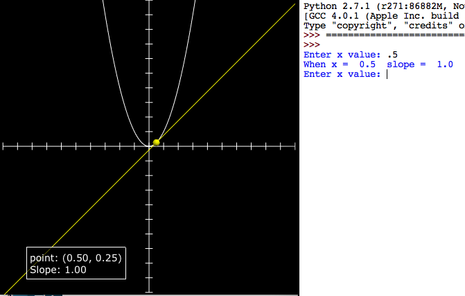
A Visual Introduction to Differentiation (using vpython)

Screen capture: Enter an x value and the program calculates the slope for the function and draws the tangent line.

This quick program is intended to introduce differentiation as a way of finding the slope of a line. Students know how to find the slope of a tangent line at least conceptually (by drawing). We pick a curve: in this case:

$f(x) = x^2$

then enter values of x in the program to see how x, the function value and the differential compare to each other.

x	f(x)	f'(x)
0.5	0.25	1
1	1	2
2	2	4
3	9	6

Because it’s quick you have to change the function in the code, and enter the values for x in the python shell.

differentiation_intro_numeric.py

from visual import *

class tangent_line:
    def __init__(self):
        self.dx = 0.1
        self.line = curve()
        self.tangent_line = curve()
        self.point = sphere(radius=.25,color=color.yellow)
        self.point.visible = False
        self.label = label(pos=(-5,-8))

    '''CHANGE FUNCTION (y) HERE'''
    # the original function
    def f(self, x):
        #y = sin(x)
        y = x**2
        return y
    '''END CHANGE FUNCTION HERE'''

    def find_slope(self, x):
        sdx = .00001
        m = (self.f(x+sdx)-self.f(x))/sdx
        return round(m,3)
        
    def draw(self):
        for x in arange(xmin, xmax+self.dx, self.dx):
            self.line.append(pos=(x, self.f(x)))

    def draw_tangent(self, x):
        m = self.find_slope(x)
        y = self.f(x)
        b = y - m * x
        print "When x = ", x, " slope = ", m
        self.label.text = "point: (%1.2f, %1.2f)\nSlope: %1.2f" % (x,y,m)
        self.plot_point(x)

        #draw tangent
        self.tangent_line.visible = False
        self.tangent_line = curve(pos=[(xmin,m*xmin+b),(xmax,m*xmax+b)], color=color.yellow)
              
    def plot_point(self, x):
        self.point.visible = True
        self.point.pos = (x, self.f(x)) 

#axes
xmin = -10.
xmax = 10.
ymin = -10.
ymax = 10.
xaxis = curve(pos=[(xmin,0),(xmax,0)])
yaxis = curve(pos=[(0,ymin),(0,ymax)])

#tick marks
tic_dx = 1.0
tic_h = .5
for i in arange(xmin,xmax+tic_dx,tic_dx):
    tic = curve(pos=[(i,-0.5*tic_h),(i,0.5*tic_h)])
for i in arange(ymin,ymax+tic_dx,tic_dx):
    tic = curve(pos=[(-0.5*tic_h,i),(0.5*tic_h,i)])

#stop scene from zooming out too far when the curve is drawn
scene.autoscale = False

# draw curve
func = tangent_line()
func.draw()

# get input
while 1:
    xin = raw_input("Enter x value: ")
    func.draw_tangent(float(xin))

Coding Online on the Coding Ground

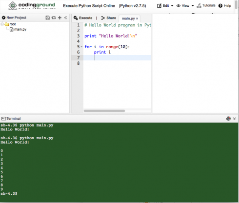
For some of my students with devices like Chromebooks, it has been a little challenging finding ways for them to do coding without a simple, built-in interpreter app. One interim option that I’ve found, and like quite a bit is the TutorialsPoint Coding Ground, which has online interfaces for quite a number of languages that are great for testing small programs, including Python.

Screen capture of Python coding at Tutorial Point's Coding Ground. — Screen capture of Python coding at Tutorial Point’s Coding Ground.