Calculating the forces between two charged particles (electric force), two magnets (the magnetic force), and two masses (the gravitational force) require remarkably similar equations. But, while electricity and magnetism are directly related (that’s why it’s called electromagnetism), gravity is its own fundamental force. Yet they all depend (inversely) on the square of the distance between the two objects creating the force, so they’re all said to obey some form of the inverse square law.
Gravitational Force (Fg)
The force exerted by two masses on one another is:
where:
G is the gravitational constant (6.67300 × 10⁻¹¹ m3 kg-1 s-2
m1 and m2 are the masses of the two objects attracting one another.
d is the distance between the two objects.
Electrical Force (Fe)
The force exerted by two electrically charged objects on one another (like a proton and an electron), is:
where:
K is the electrical constant, sometimes called Coulumn’s constant (8.9876 × 10⁹ N m2 C-2
q1 and q2 are the sizes of the charges (in Coulumbs) of the two objects attracting one another.
d is the distance between the two objects.
Magnetic Force (Fm)
The force exerted by two magnets on one another, is:
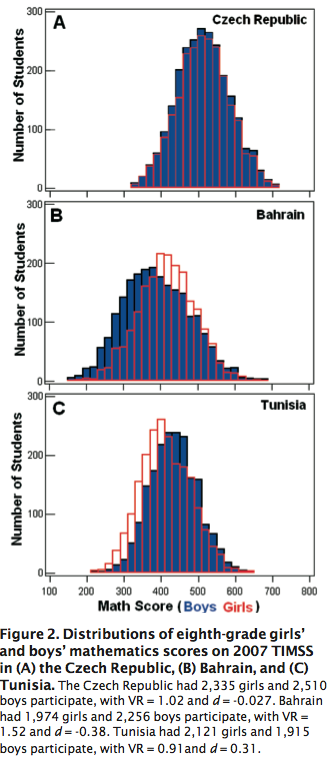
Boys tend to be better at math. That’s been the stereotype, but a new study (Kane and Mertz, 2011) published in the Notices of the American Mathematical Society provides evidence that, at all levels, it’s only because society and culture tend to support, and advance the stereotype.
… we conclude that gender equity and other sociocultural factors, not national income, school type, or religion per se, are the primary determinants of mathematics performance at all levels for both boys and girls. … It is fully consistent with socioeconomic status of the home environment being a primary determinant for success of children in school.
Kane and Mertz compared math achievement in a number of countries. If there were some genetic reason for different math abilities then boys should be better than girls everywhere. This is not the case. In more wealthy countries where there is more equality between the genders, the mathematics performance gap disappears.
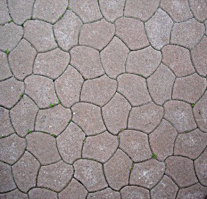
The Missouri Council of Teachers of Mathematics (MoCTM) has a Math & Art Contest that focuses on Geometry. It has fairly simple expectations, and it’s aimed at Middle School students and lower. The tie between the math and the art does not require much depth, but that’s probably appropriate for students who are still developing abstract thinking.
I’m usually a bit cautious about the utility of contests. Their primary benefit is in the work that they motivate, not the reward (or hope of a reward) at the end; although, students do need to learn to win or lose with equanimity.
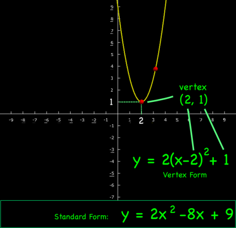
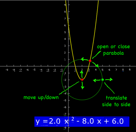
So I put together this interactive parabola program using VPython (code here) for students encountering these curves in Algebra.
It’s a more interactive version of the Excel parabola program in that you can move the curve by dragging on some control points, rather than just having to enter the coefficients of the equation. The program is still in development, but it is at a useful stage right now, so I thought I’d make it available for anyone who wanted to try it.
The program is fairly straightforward to use. You can move the curve (translate it) up and down, and expand or tighten the area within the parabola.
The program also displays the equation of the curve in standard form:
.
Next Steps
I’m also working making the standard equation editable by clicking on it and typing, and am considering showing the x-axis intercepts, which will give algebra students a nice, visual way to of checking their factoring.
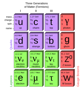
When it comes to particle physics … [m]easuring something once is meaningless because of the high degree of uncertainty involved in such exotic, small systems. Scientists rely on taking measurements over and over again — enough times to dismiss the chance of a fluke.
New research, out of the Large Haldron Collider in Switzerland, shows a 0.8% difference in the way matter and antimatter particles behave. This small difference could go a long way in explaining why the universe is made up mostly of matter today, even though in the beginning there were about equal amounts of matter and antimatter. It would mean that the current, best theory describing particle physics, the Standard Model, needs some significant tweaking.
0.8% is small, but significant. How confident are the physicists that their measurements are accurate? Well, the more measurements you take the more confident you can be in your average result, though you can never be 100% certain. The LHC scientists did enough measurements that they could calculate, statistically, that there is only a 0.05% chance that their measurement is wrong.
visual.ly posts and hosts some excellent graphics. The one below, calculates the nearly infinitesimal probability of just being born. There’s hardly a better argument for appreciating life.
It’s also a good example of working with probabilities [and] exponents. Very large exponents.
A series of still photographs of a projectile (soccer ball) in motion were used to determine the equation for the height of the ball (h(t) = 4.9 t2 + 14.2 t + 1.25), the initial velocity of the ball (14.2 m), the maximum height of the ball (11.6 m), and the time between each photograph (0.41 s). The problem was solved numerically using MS Excel’s Solver function. There are much easier ways of doing this, which we did not do.
Introduction
One of physics lab assignments I gave my students was to see if students could use a camera to capture a sequence of images of a projectile, plot the elevation of the projectile from the photographs, determine the constants in the parabolic equation for the height of the projectile, and, in so doing, determine the velocity at which the projectile was launched.
I offered my old, digital Pentax SLR that can take up to seven pictures in quick sequence and be set to fully manual. A digital video camera with a detailed timestamp would have been ideal, but we did not have one available at the time.
Now the easy way of getting the velocity data would be to estimate the heights (h) of the ball from the image using some sort of known reference (in this case the whiteboard), and determine the time between each photograph (Δt) by photographing a stopwatch using the same shutterspeed settings. After all, the average velocity of the ball between two images would be:
The reference whiteboard is four feet tall (1.22 m) in real life, but 51 pixels tall in the image. Using this ratio (i.e. 1.22 m = 51 px) we can convert the heights of the ball from pixels to meters:
Unfortunately, I think my students forgot to do the pictures of the stopwatch to get Δt, the time between each photograph. Since the lab reports are due on Monday, and it’s the weekend now I’m curious to see what they come up with.
However, I was wondering if they could use just the elevation data to back out the Δt. So I gave it a try myself. Even the easiest way of solving this problem is not trivial, in fact, I ended up resorting to Excel’s iterative solver to find the answers. While this procedure probably goes a little beyond what I expect from the typical high school physics student, more advanced students who are taking calculus might benefit.
Procedure
We took the reference whiteboard (1.21 m tall), a soccer ball, and the camera outside. The whiteboard was leant vertically against the post of the soccer goal. The ball was thrown vertically by a student standing next to the whiteboard (see Figure 1) while pictures were taken. The camera’s shutterspeed was 1/250th of a second. The distance from the camera to the person throwing the ball (and to the whiteboard) were not measured.
The procedure was repeated several times, but only one trail was used in this analysis.
The images were loaded onto a computer, and the program GIMP was used to determine the distance, in pixels, from the ground to the projectile. The size of the reference whiteboard, in pixels, was used to calculate the height of the soccer ball in meters.
The elevations measured off the photographs were then used to calculate the release velocity, time between snapshots, and maximum height of the ball.
The Equation for Elevation
I started with the fact that once the ball is released, the only force acting on it is the force of gravity. Since the mass of the ball does not change we only have to consider the acceleration due to gravity (-9.8 m/s2). I also neglect air resistance to make things easier.
Finding the Velocity Equation
Start with the fact that, acceleration is the rate of change of velocity with time. You can write it in the differential form:
so we integrate with respect to time to get the equation for velocity as a function of time:
where c is an unknown constant. What we do know though, is that at the beginning, when the ball is just launched, time is zero (t = 0) so cv becomes the initial velocity (v0) at which the ball is thrown:
at t = 0, v(0) = v0:
So our velocity equation becomes:
Finding the height equation
Now since we know that velocity is the rate of change of distance (in this case height) with time:
so we integrate again to find the height equation:
Similar to what we did with the velocity equation, to find the new constant c we consider what happens at the start time, when the ball is launched, and t = 0 and h(0) = h0;
so:
The constant is equal to the initial height of the ball — the height of the ball when it’s thrown. So we end up with the final equation:
Results
Solving all the unknowns
At this point, although we have an equation for the height of the ball, we don’t know the initial velocity (v0), nor do we know the initial height of the ball when it’s released (h0). And we still don’t know the time when the ball is at each position.
With that many unknowns we’d need the same number of independent equations to be able to solve for them all. It may be possible, but instead of analytically solving the equations I opted to take a numerical approach, and use Excel’s Solver function.
I started by setting up the equations to calculate the height of the ball at six different times to correspond with our six height measurements. It was necessary therefore to create a set of variables:
Time when we started taking pictures (t1): Since we don’t know how long after we threw the ball we started taking pictures, I made this a variable called t1.
The time between each picture (dt): I made the assumption that the time between each picture would be constant. The shutter speed was constant (1/250th of a second) so there is no obvious reason why the time should be different.
Initial velocity (v0): The initial upward speed at which the ball was thrown. Obviously, the faster the initial speed the higher the ball goes, so this is a fairly important parameter.
Initial height (h0): We also don’t precisely know how high the ball was when it was released, so this also needs to be a variable.
By defining the time between each picture as dt, we can write the time that each picture was taken in terms of the time of the initial picture (t1) and dt. After all the second picture would have been taken dt seconds after the first for a total time of:
similarly for all the pictures:
Now I set up an Excel spreadsheet and gave all the unknown variable values and initial value of 1:
Now I just had to run Solver and tell it that I wanted the Total Residual, which gives the difference between the h(1) equation’s values for height and the actual, measured values, to be as close to zero as possible. A perfect fit of the equation to the data would have a total residual of one, but that’s not possible when you’re dealing with real data.
Even so, I had to goose Solver a bit for it to produce reasonable numbers. I put in a few constraints:
dt >= 0: We could not have a negative time between pictures.
h0 <= 1.25: 1.25 meters seemed reasonable for the height at which the ball was released.
t1 <= 1: It also seemed reasonable that the time when the first picture was taken was less than one second after the ball was thrown.
I ran the Solver a few times, and had to reset dt to 0.5 at one point when it had become zero, but the final result looked remarkably good: the total difference between the modeled line and the actual data was only 0.113 meters.
So we found that:
Initial velocity: v0 = 14.2 m/s
Height at release: h0 = 1.25 m
Time between pictures: dt = 0.41 s
Time when the first picture was taken: t1 = 0.44 s
Which makes the height equation:
Using these constants in the height equation, we could see how good fit the height equation was to the data:
Maximum Height of the Ball
Finally, the maximum height of the ball can be read off the graph, but it can also be determined using the equation for the height of the ball:
We know that the maximum height is reached when the ball stops moving upward and starts to descend. At that point, the vertical velocity of the ball is zero. Since the velocity of the ball is the rate of change of height () we can differentiate the height equation to get an equation for velocity.
since we’ve determined that the initial velocity of the ball is 14.2 m/s we get:
when the velocity is zero (v = 0):
which can be solved for t to find that the time the ball reaches it’s maximum height is:
Putting this into the height equation:
gives:
Discussion
I’m quite happy with the way this project turned out. The fit between the modeled heights (h(t)) and the actual heights was very good.
My primary concern going into the project was that the distortion from the camera lens would make this technique impossible, but that appears not to be a significant problem.
Most of this calculation, including the somewhat tricky numerical solution using Solver could have been avoided if I’d calibrated the camera, simply by pointing it at a stopwatch (using the same shutterspeed as in the experiment) and measuring the time between snapshots. It will therefore be interesting to see if the actual time between shots (dt) is close to the dt of 0.41 seconds calculated by the model.
Finally, as noted above, a video camera with a timestamp would possibly be a more useful technology for this experiment.
Conclusion
It is possible to analyze the projectile path of an object using a series of snapshots, to determine the initial velocity of the projectile, its release height, and the time between snapshots, if you can assume that the time between snapshots is identical. There are, however, much easier methods of solving this problem.