Mathematics – Page 3 – Montessori Muddle

Maximum Range of a Potato Gun

One of the middle schoolers built a potato gun for his math class. He was looking a the mathematical relationship between the amount of fuel (hair spray) and the hang-time of the potato. To augment this work, I had my Numerical Methods class do the math and create analytical and numerical models of the projectile motion.

One of the things my students had to figure out was what angle would give the maximum range of the projectile? You can figure this out analytically by finding the function for how the horizontal distance (x) changes as the angle (theta) changes (i.e. x(theta)) and then finding the maximum of the function.

Initial velocity vector (v) and its component vectors in the x and y directions. — Initial velocity vector (v) and its component vectors in the x and y directions for a given angle.

Distance as a function of the angle

In a nutshell, to find the distance traveled by the potato we break its initial velocity into its x and y components (v_x and v_y), use the y component to find the flight time of the projectile (t_f), and then use the v_x component to find the distance traveled over the flight time.

Starting with the diagram above we can separate the initial velocity of the potato into its two components using basic trigonometry:

$\cos{\theta} = \frac{v_x}{v}$
$\sin{\theta} = \frac{v_y}{v}$ ,

so,

$v_x = v \cos{\theta}$ ,
$v_y = v \sin{\theta}$

Now we know that the height of a projectile (y) is given by the function:

$! y(t) = \frac{a t^2}{2} + v_0 t + y_0$

(you can figure this out by assuming that the acceleration due to gravity (a) is constant and acceleration is the second differential of position with respect to time.)

To find the flight time we assume we’re starting with an initial height of zero (y₀ = 0), and that the flight ends when the potato hits the ground which is also at zero ((y_t = 0), so:

$! 0 = \frac{a t^2}{2} + v_0 t + 0$

$! 0 = \frac{a t^2}{2} + v_0 t$

Factoring out t gives:

$! 0 = t ( \frac{a t}{2} + v_0)$

Looking at the two factors, we can now see that there are two solutions to this problem, which should not be too much of a surprise since the height equation is parabolic (a second order polynomial). The solutions are when:

$! t = 0$

$! \frac{a t}{2} + v_0 = 0$

The first solution is obviously the initial launch time, while the second is going to be the flight time (t_f).

$! \frac{a t_f}{2} + v_0 = 0$

$! t_f = - \frac{2 v_0}{a}$

You might think it’s odd to have a negative in the equation, but remember, the acceleration is negative so it’ll cancel out.

Now since we’re working with the y component of the velocity vector, the initial velocity in this equation (v₀) is really just v_y:

$! v_0 = v_y$

so we can substitute in the trig function for v_y to get:

$! t_f = - \frac{2 v \sin{\theta}}{a}$

Our horizontal distance is simply given by the velocity in the x direction (v_x) times the flight time:

$! x = v_x t_f$

which becomes:

$! x = v_x \left(- \frac{2 v \sin{\theta}}{a}\right)$

and substituting in the trig function for v_x (just to make things look more complicated):

$! x = \left( v \cos{\theta} \right) \left(- \frac{2 v \sin{\theta}}{a}\right)$

and factoring out some of the constants gives:

$! x = -\frac{v^2}{a} 2 \sin{\theta}\cos{theta}$

Now we have distance as a function of the launch angle.

We can simplify this a little by using the double-angle formula:

$! \sin{2\theta} = 2 \sin{\theta}\cos{theta}$

to get:

$! x = -\frac{v^2}{a} \sin{2\theta}$

Finding the maximum distance

How do we find the maxima for this function. Sketching the curve should be easy enough, but because we know a little calculus we know that the maximum will occur when the first differential is equal to zero. So we differentiate with respect to the angle to get:

$! \frac{dx}{d\theta} = -\frac{v^2}{a} 2 \cos{2\theta}$

and set the differential equal to zero:

$! 0 = -\frac{v^2}{a} 2 \cos{2\theta}$

and solve to get:

$! \cos{2\theta} = 0$

$! 2\theta = \cos^{-1}{(0)}$

Since we remember that the arccosine of 0 is 90 degrees:

$! 2\theta = 90^{\circ}$

$! \theta = 45^{\circ}$

And thus we’ve found the angle that gives the maximum launch distance for a potato gun.

Spurious Correlations

Tyler Vigen has a great website Spurious Correlations that shows graphs of exactly that.

Great for explaining what correlation means, and why correlation does not necessarily mean causation.

Numerical and Analytical Solutions 2: Constant Acceleration

Previously, I showed how to solve a simple problem of motion at a constant velocity analytically and numerically. Because of the nature of the problem both solutions gave the same result. Now we’ll try a constant acceleration problem which should highlight some of the key differences between the two approaches, particularly the tradeoffs you must make when using numerical approaches.

The Problem

A ball starts at the origin and moves horizontally with an acceleration of 0.2 m/s². Print out a table of the ball’s position (in x) with time (every second) for the first 20 seconds.

Analytical Solution
We know that acceleration (a) is the change in velocity with time (t):

$a = \frac{dv}{dt}$

so if we integrate acceleration we can find the velocity. Then, as we saw before, velocity (v) is the change in position with time:

$v = \frac{dx}{dt}$

which can be integrated to find the position (x) as a function of time.

So, to summarize, to find position as a function of time given only an acceleration, we need to integrate twice: first to get velocity then to get x.

For this problem where the acceleration is a constant 0.2 m/s² we start with acceleration:

$\frac{dv}{dt} = 0.2$

which integrates to give the general solution,

$v = 0.2 t + c$

To find the constant of integration we refer to the original question which does not say anything about velocity, so we assume that the initial velocity was 0: i.e.:

at t = 0 we have v = 0;

which we can substitute into the velocity equation to find that, for this problem, c is zero:

$v = 0.2 t + c$
$0 = 0.2 (0) + c$
$0 = c$

making the specific velocity equation:
$v = 0.2 t$

we replace v with dx/dt and integrate:

$\frac{dx}{dt} = 0.2 t$
$x = \frac{0.2 t^2}{2} + c$
$x = 0.1 t^2 + c$

This constant of integration can be found since we know that the ball starts at the origin so

at t = 0 we have x = 0, so;

$x = 0.1 t^2 + c$
$0 = 0.1 (0)^2 + c$
$0 = c$

Therefore our final equation for x is:

$x = 0.1 t^2$

Summarizing the Analytical

To summarize the analytical solution:

$a = 0.2$
$v = 0.2 t$
$x = 0.1 t^2$

These are all a function of time so it might be more proper to write them as:

$a(t) = 0.2$
$v(t) = 0.2 t$
$x(t) = 0.1 t^2$

Velocity and acceleration represent rates of change which so we could also write these equations as:

$a(t) = \frac{dv}{dt} = 0.2$
$v(t) = \frac{dx}{dt} = 0.2 t$
$x(t) = x = 0.1 t^2$

or we could even write acceleration as the second differential of the position:

$a(t) = \frac{d^2x}{dt^2} = 0.2$
$v(t) = \frac{dx}{dt} = 0.2 t$
$x(t) = x = 0.1 t^2$

or, if we preferred, we could even write it in prime notation for the differentials:

$a(t) = x''(t) = 0.2$
$v(t) = x'(t) = 0.2 t$
$x(t) = x(t) =0.1 t^2$

The Numerical Solution

As we saw before we can determine the position of a moving object if we know its old position (x_old) and how much that position has changed (dx).

$x_{new} = x_{old} + dx$

where the change in position is determined from the fact that velocity (v) is the change in position with time (dx/dt):

$v = \frac{dx}{dt}$

which rearranges to:

$dx = v dt$

So to find the new position of an object across a timestep we need two equations:

$dx = v dt$
$x_{new} = x_{old} + dx$

In this problem we don’t yet have the velocity because it changes with time, but we could use the exact same logic to find velocity since acceleration (a) is the change in velocity with time (dv/dt):

$a = \frac{dv}{dt}$

which rearranges to:

$dv = a dt$

and knowing the change in velocity (dv) we can find the velocity using:

$v_{new} = v_{old} + dv$

Therefore, we have four equations to find the position of an accelerating object (note that in the third equation I’ve replaced v with v_new which is calculated in the second equation):

$dv = a dt$
$v_{new} = v_{old} + dv$
$dx = v_{new} dt$
$x_{new} = x_{old} + dx$

These we can plug into a python program just so:

motion-01-both.py

from visual import *

# Initialize
x = 0.0
v = 0.0
a = 0.2
dt = 1.0

# Time loop
for t in arange(dt, 20+dt, dt):

     # Analytical solution
     x_a = 0.1 * t**2

     # Numerical solution
     dv = a * dt
     v = v + dv
     dx = v * dt
     x = x + dx

     # Output
     print t, x_a, x

which give output of:

>>> 
1.0 0.1 0.2
2.0 0.4 0.6
3.0 0.9 1.2
4.0 1.6 2.0
5.0 2.5 3.0
6.0 3.6 4.2
7.0 4.9 5.6
8.0 6.4 7.2
9.0 8.1 9.0
10.0 10.0 11.0
11.0 12.1 13.2
12.0 14.4 15.6
13.0 16.9 18.2
14.0 19.6 21.0
15.0 22.5 24.0
16.0 25.6 27.2
17.0 28.9 30.6
18.0 32.4 34.2
19.0 36.1 38.0
20.0 40.0 42.0

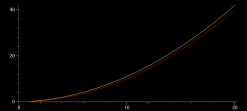
Here, unlike the case with constant velocity, the two methods give slightly different results. The analytical solution is the correct one, so we’ll use it for reference. The numerical solution is off because it does not fully account for the continuous nature of the acceleration: we update the velocity ever timestep (every 1 second), so the velocity changes in chunks.

To get a better result we can reduce the timestep. Using dt = 0.1 gives final results of:

18.8 35.344 35.532
18.9 35.721 35.91
19.0 36.1 36.29
19.1 36.481 36.672
19.2 36.864 37.056
19.3 37.249 37.442
19.4 37.636 37.83
19.5 38.025 38.22
19.6 38.416 38.612
19.7 38.809 39.006
19.8 39.204 39.402
19.9 39.601 39.8
20.0 40.0 40.2

which is much closer, but requires a bit more runtime on the computer. And this is the key tradeoff with numerical solutions: greater accuracy requires smaller timesteps which results in longer runtimes on the computer.

Post Script

To generate a graph of the data use the code:

from visual import *
from visual.graph import *

# Initialize
x = 0.0
v = 0.0
a = 0.2
dt = 1.0

analyticCurve = gcurve(color=color.red)
numericCurve = gcurve(color=color.yellow)
# Time loop
for t in arange(dt, 20+dt, dt):

     # Analytical solution
     x_a = 0.1 * t**2

     # Numerical solution
     dv = a * dt
     v = v + dv
     dx = v * dt
     x = x + dx

     # Output
     print t, x_a, x
     analyticCurve.plot(pos=(t, x_a))
     numericCurve.plot(pos=(t,x))

which gives:

Comparison of numerical and analytical solutions using a timestep (dt) of 1.0 seconds.

Numerical versus Analytical Solutions

We’ve started working on the physics of motion in my programming class, and really it boils down to solving differential equations using numerical methods. Since the class has a calculus co-requisite I thought a good way to approach teaching this would be to first have the solve the basic equations for motion (velocity and acceleration) analytically–using calculus–before we took the numerical approach.

Constant velocity

Question 1. A ball starts at the origin and moves horizontally at a speed of 0.5 m/s. Print out a table of the ball’s position (in x) with time (t) (every second) for the first 20 seconds.

Analytical Solution:
Well, we know that speed is the change in position (in the x direction in this case) with time, so a constant velocity of 0.5 m/s can be written as the differential equation:

$\frac{dx}{dt} = 0.5$

To get the ball’s position at a given time we need to integrate this differential equation. It turns out that my calculus students had not gotten to integration yet. So I gave them the 5 minute version, which they were able to pick up pretty quickly since integration’s just the reverse of differentiation, and we were able to move on.

Integrating gives:

$x = 0.5t + c$

which includes a constant of integration (c). This is the general solution to the differential equation. It’s called the general solution because we still can’t use it since we don’t know what c is. We need to find the specific solution for this particular problem.

In order to find c we need to know the actual position of the ball is at one point in time. Fortunately, the problem states that the ball starts at the origin where x=0 so we know that:

at t = 0, x = 0

So we plug these values into the general solution to get:

$0 = 0.5(0) + c$
solving for c gives:

$c = 0$

Therefore our specific solution is simply:

$x = 0.5t$

And we can write a simple python program to print out the position of the ball every second for 20 seconds:

motion-01-analytic.py

for t in range(21):
     x = 0.5 * t
     print t, x

which gives the result:

Numerical Solution:
Finding the numerical solution to the differential equation involves not integrating, which is particularly good if the differential equation can’t be integrated.

We start with the same differential equation for velocity:
$\frac{dx}{dt} = 0.5$

but instead of trying to solve it we’ll just approximate a solution by recognizing that we use dx/dy to represent when the change in x and t are really, really small. If we were to assume they weren’t infinitesimally small we would rewrite the equations using deltas instead of d’s:
$\frac{\Delta x}{\Delta t} = 0.5$

now we can manipulate this equation using algebra to show that:
$\Delta x = 0.5 \Delta t$

so the change in the position at any given moment is just the velocity (0.5 m/s) times the timestep. Therefore, to keep track of the position of the ball we need to just add the change in position to the old position of the ball:

$x_{new} = x_{old} + \Delta x$

Now we can write a program to calculate the position of the ball using this numerical approximation.

motion-01-numeric.py

from visual import *

# Initialize
x = 0.0
dt = 1.0

# Time loop
for t in arange(dt, 21, dt):
     v = 0.5
     dx = v * dt
     x = x + dx
     print t, x

I’m sure you’ve noticed a couple inefficiencies in this program. Primarily, that the velocity v, which is a constant, is set inside the loop, which just means it’s reset to the same value every time the loop loops. However, I’m putting it in there because when we get working on acceleration the velocity will change with time.

I also import the visual library (vpython.org) because it imports the numpy library and we’ll be creating and moving 3d balls in a little bit as well.

Finally, the two statements for calculating dx and x could easily be combined into one. I’m only keeping them separate to be consistent with the math described above.

A Program with both Analytical and Numerical Solutions
For constant velocity problems the numerical approach gives the same results as the analytical solution, but that’s most definitely not going to be the case in the future, so to compare the two results more easily we can combine the two programs into one:

motion-01.py

from visual import *
# Initialize
x = 0.0
dt = 1.0

# Time loop
for t in arange(dt, 21, dt):
     v = 0.5

     # Analytical solution
     x_a = v * t

     # Numerical solution
     dx = v * dt
     x = x + dx

     # Output
     print t, x_a, x

which outputs:

>>> 
1.0 0.5 0.5
2.0 1.0 1.0
3.0 1.5 1.5
4.0 2.0 2.0
5.0 2.5 2.5
6.0 3.0 3.0
7.0 3.5 3.5
8.0 4.0 4.0
9.0 4.5 4.5
10.0 5.0 5.0
11.0 5.5 5.5
12.0 6.0 6.0
13.0 6.5 6.5
14.0 7.0 7.0
15.0 7.5 7.5
16.0 8.0 8.0
17.0 8.5 8.5
18.0 9.0 9.0
19.0 9.5 9.5
20.0 10.0 10.0

Solving a problem involving acceleration comes next.

Model Skate Park

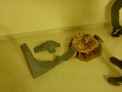
After batting around a number of ideas, three of my middle schoolers settled on building a model skate park out of popsicle sticks and cardboard for their interim project.

A lot of hot glue was involved.

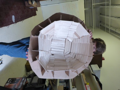
The ramps turned out to be pretty easy, but on the second day they decided that the wanted a bowl, which proved to be much more challenging. They cut out sixteen profiles out of thicker cardboard, made a skeleton out of popsicle sticks, and then coated the top with thin, cereal-box cardboard.

When they were done they painted the whole thing grey–to simulate concrete I think–except for the sides, which were a nice flat blue so that they could put their own miniature graffiti over the top.

It was a lot of careful, well thought-out work.

Gaga Ball Pit

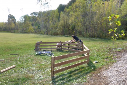
A couple middle-schoolers decided to build a gaga ball pit for their interim project. Since they’d already had their plan improved and I’d picked up the wood over the weekend, they figured they could get it done in a day or two and then move on to other things for the rest of the week. However, it turned out to be a bit more involved.

They spent most of their first day–they just had afternoons to work on this project–figuring out where to build the thing. It’s pretty large, and our head-of-school was in meetings all afternoon, so there was a lot of running back and forth.

The second day involved some math. Figuring out where to put the posts required a little geometry to determine the internal angles of an octagon, and some algebra (including Pythagoras’ Theorem) to calculate the distance across the pit. The sum a² + a² proved to be a problem, but now that they’ve had to do it in practice they won’t easily forget that it’s not a⁴.

Mounting the rails on the posts turned out the be the main challenge on day three. They initially opted for trying to drill the rails in at an angle, but found out pretty quickly that that was going to be extremely difficult. Eventually, they decided to rip the posts at a 45 degree angle to get the 135 degree outer angle they needed. We ran out of battery power for the saw and our lag screws were too long for the new design, so assembly would have to wait another day.

Finally, on day four they put the pit together. It only took about an hour–they’d had the great idea on day three to put screws into the posts at the right height, so that they could rest the rails on the screws to hold them into place temporarily as they mounted the rails. By the time they added the final side the octagon was only off by a few, easily adjusted centimeters.

They did an excellent job and noted, in our debrief, just how important the planning was, even though it was their least favorite part of the project. I’d call it a successful project.

Some Geometry in Archery

Our PE teacher just started up an archery program at school (first classes today actually), and she shared this video with me that seems like it might be useful in geometry class. Specifically, it uses circle packing to estimate the relative difficulty for an archer to hit different sized circular targets.

Volumes of Revolution

It can be tricky explaining what you mean when you say to take a function and rotate it about the x-axis to create a volume. So, I made an OpenScad program to make 3d prints of functions, including having it subtract one function from another. I also 3d printed a set of axes to mount the volumes on (and a set of cross-sections of the volumes being rotated.

The picture above are the functions Mrs. C. gave her calculus class on a recent worksheet. Specifically:

$y = e^{-x}+2$

from which is subtracted:

$y = 0.5 x$