Algebra and Programming with VPython

Computer programming is the place where algebra comes to life. Students seem to get really excited when they write even the simplest instructions and see the output on the screen. I’m not sure exactly why this is the case, but I suspect it has something to do with being able to see the transition from abstract programming instructions to “concrete” results.

So I’ve decided to supplement my Algebra classes with an introduction to programming. I’m using the Python programming language, or, more specifically, the VPython variant of the language.

Why VPython? Because it’s free, it’s an easy-to-use high-level language, and it’s designed for 3d output, which seems to be somewhat popular these days. The oohs and aahs of seeing the computer print the result of a+b turn into wows when they create their first box. I’ve used the language quite a bit myself, and there are a lot of other interesting applications available if you search the web.

VPython was created to help with undergraduate physics classes, but since it was made to be usable by non-science majors, it’s really easy for middle and high school students to pick up. In fact, NCSU also has a distance education course for high school physics teachers. They also have some instructional videos available on YouTube that provide a basic introduction.
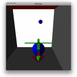
Image from a game created by middle school student Ryan W.

I use VPython models for demonstrations in my science classes, I’ve had middle school students use it for science projects, and I’ve just started my middle school algebra/pre-algebra students learning it as a programming language and they’re doing very well so far.

What I hope to document here is the series of lessons I’m putting together to tie, primarily, into my middle school algebra class, but should be useful as a general introduction to programming using VPython.

Getting VPython

You’ll need to install Python and VPython on your system. They can be directly downloaded from the VPython website’s download page for Windows, Macintosh or LINUX.

Running a Python program.

Once they’re installed, you’ll have the IDLE (or VIDLE) program somewhere on your system; a short-cut is usually put on the desktop of your Windows system. Run (double-click) this program and the VPython programming editor will pop up any you’re ready to go. You can test it by typing in something simple like:

a = 1
b = 2
c = a + b
print c

Then you run the program by going through the Run–>Run Module in the menu bar.

Which should cause a new window to pop up with:

Python 2.7.1 (r271:86882M, Nov 30 2010, 09:39:13) 
[GCC 4.0.1 (Apple Inc. build 5494)] on darwin
Type "copyright", "credits" or "license()" for more information.
>>> ================================ RESTART ================================
>>> 
3
>>> 

Even better might be to test the 3d rendering, which you can do with the following program:

from visual import *

box()

which creates the following exciting image:

A box created with VPython. It looks much more interesting if you rotate it to see it in perspective.

To rotate the view, hold down and drag the right mouse button. To zoom in or out, hold down the right and left buttons together and drag in and out.
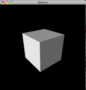
A rotated, zoomed-out view of a box.

Lessons

Lesson 1: Variables, Basic Operations, Real and Integer Numbers and the First Box.

Lesson 2: Creating a graphical calculator: Coordinates, lists, loops and arrays: A Study in Linear Equations
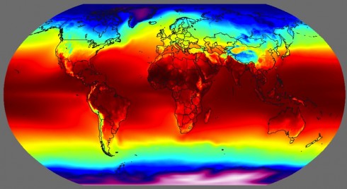
Global Warming Art

Global temperatures (averaged from 1961-1990). Image created for Global Warming Art by Robert A. Rohde.

Talk about evoking conflicting emotions. The image is astoundingly beautiful – I particularly like the rich, intense colors – but the subject, global warming, always leaves me with sense of apprehension since it seems so unlikely that enough will be done to ameliorate it.

The source of the image, Global Warming Art has a number of excellent images, diagrams and figures. The National Oceanic and Atmospheric Administration also has lots of beautiful, weather-related diagrams. I particularly like the seasonal temperature change animation I made from their data.

The Thermal Difference Between Land and Water

The change in temperatures over the course of the year. Click image to enlarge. Images from 1987 via NOAA's GLOBE Earth System Poster.

The continents heat up faster than the oceans, and they cool down faster too. You can see this quite clearly in the animation above: notice how cold North America gets in the winter compared to the North Atlantic. It’s why London has an average January low temperature of 2˚C while Winnepeg’s is closer to -20˚C, even though they’re at almost the same latitude. There are a few reasons for the land-ocean cooling differences, and they all have to do with how heat is absorbed and transported.

(1) Specific Heat Capacity. Water has a higher heat capacity than land. So it takes more heat to raise the temperature of one gram of water by one degree than it does to raise the temperature of land. 1 calorie of solar energy (any type of energy really) will warm one gram of water by 1 degree Celcius, while the same calorie would raise the temperature of a gram of granite by more than 5 degrees C. The Engineering Toolbox has specific heat capacities of common materials.

(2) Transparency. The heat absorbed by the ocean is spread out over a greater volume because the oceans are transparent (to some degree). Since light can penetrate the surface of the water the heat from the sun is dispersed over a greater depth.

(3) Evaporation. The oceans loose a lot of heat from evaporation. In the evaporative heat loss experiment, While there is some evaporation from wet soils and transpiration by plants, the land does not have anywhere near as much available moisture to cool it down.

(4) Currents. Not only do the oceans absorb heat over a greater depth, but they can also move that energy around with their currents. The solar energy absorbed at the equator gets transported towards the poles, while the colder polar water gets transported the other way. Currents help average out ocean temperatures.

The Freezing Core Keeps the Earth Warm

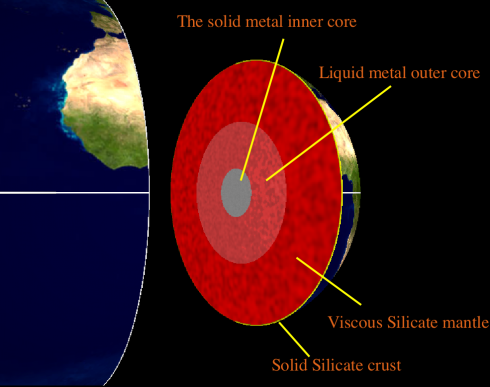
The internal structure of the Earth.

The inner core of the Earth is made of solid metal, mostly iron. The outer core is also made of metal, but it’s liquid. Since it formed from the solar nebula, our planet has been cooling down, and the outer core has been freezing onto the inner core. Somewhat counter-intuitively, the freezing process is a phase change that releases energy – after all, if you think about it, it takes energy to melt ice.

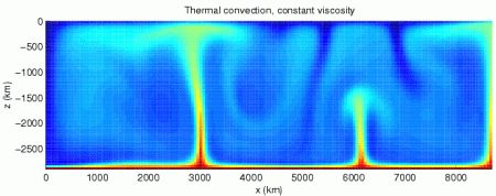
The energy released from the freezing core is transported upward through the Earth’s mantle by convection currents, much like the way water (or jam) circulates in a boiling pot. These circulating currents are powerful enough to move the tectonic plates that make up the crust of the earth, making them responsible for the shape and locations of the mountain ranges and ocean basins on the Earth’s surface, as well as the earthquakes and volcanics that occur at plate boundaries.

Conceptual drawing of assumed convection cells in the mantle. (via The Dynamic Earth from the USGS).

Eventually, the entire inside of the earth will solidify, the latent heat of fusion will stop being released, and tectonics at the surface will slow to a stop.

The topic came up when we were talking about the what heats the Earth. Although most of the energy at the surface comes from solar radiation, students often think first of the heat from volcanoes.

Note: An interesting study recently published showed that although the core outer core is mostly melting, in some places it’s freezing at the same time. Unsurprising given the convective circulation in the mantle.

Model of convection in the Earth's mantle. Notice that some areas on the mantle are hotter, creating hot plumes, and some are cooler (image from Wikipedia).

Note 2: Convection in the liquid outer core is what’s responsible for the Earth’s magnetic field, and explains why the magnetic polarity (north-south) switches occasionally. We’ll revisit this when we talk about electricity and dynamos.

The (almost) Perfect Teacup

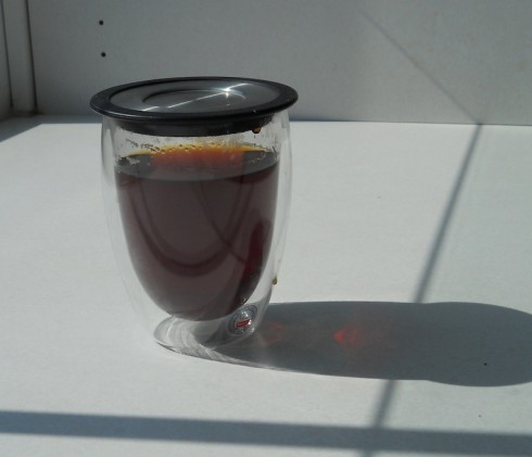
It’s a glass really. Double walled, liquid suspended in air, beautiful to look at. But it really becomes a wondrous artifact of engineering when its combined with the heavy, rubber and stainless steel lid. The beauty and thermal efficacy of this tea-making system is … elegant. It’s certainly a worthy starting point for our discussion of heat, temperature and thermodynamics in general, and generates interesting questions about heat transport (convective, evaporative, conductive and radiative) and the greenhouse effect, that can be tested with relatively simple experiments.

The first, and most obvious thing my students observed was the fact that the lid prevented heat escaping. The weight of the lid confines the head space, which reduces convective heat loss above the cup and increases the vapor pressure, which reduces the amount of tea that evaporates. Evaporation is the primary way heat is lost from hot liquids, since each gram that evaporates takes 540 calories of heat with it. A simple evaporative heat loss experiment showed that about 70% of the cooling of a cup of water came from evaporation.

The second thing the students pointed out is that the double walled glass insulates, because it reduces conductive heat loss. Solid glass has a thermal conductivity of about 0.24 cal/(s.m.K) (Engineering Toolbox.com; 1 J = 0.24 calories). The conductivity of the air in the space between the walls is two orders of magnitude less at 0.0057 cal/(s.m.K). Of course, having a vacuum in the space would be even better, but it would test the strength of the glass.

Thermally, the glass falls short when it comes to radiative heat loss. A silvery coating would reflect radiated heat back into the cup much better than transparent glass. However, silica glass is relatively opaque to infra-red, which should reduce radiated heat emission. A simple experiment, comparing the cooling rates of water a glass flask wrapped in aluminum foil to one without the foil should give some indication if radiative heat loss is significant.

Finally, the glass does have a thermal advantage though, via the greenhouse effect. Because it is transparent to short, high-energy wavelengths of light, like that of sunlight, but blocks the longer wavelengths of heat energy, the glass should be able to capture some heat from sunlight. This can also be experimentally tested with a couple flasks in the sun. It would be interesting to find out how any greenhouse warming compares to the radiative heat loss through the glass walls.

Last week my students did some basic observations and came up with their own experiments. Then they learned a little about thermodyamics from reading the textbook. This week, we’ll try to get a little more quantitative with the experiments and applications of what they know, and it should be interesting to see if what they’ve learned has changed the way they observe the common objects around them.

Evaporative Heat Loss from a Cup Experiment

This simple experiment was devised to estimate just how much heat is lost from a teacup due to evaporation as compared to the other types of heat loss (conduction and convection).

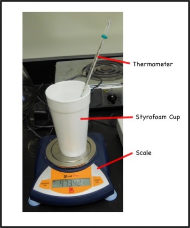
Experimental setup for measuring evaporative heat loss.

The idea is that if we can measure the mass of water that evaporates over a short period of time, we can calculate the evaporative heat loss because we know that the amount of heat it takes to evaporate one gram of water (its latent heat of evaporation) is 540 cal/g. So we’ll take some hot, almost boiling, water and weigh and take its temperature as it cools down.

Materials

Apparatus.

It requires:

  • A thermometer (Celcius up to 100 degrees)
  • A styrofoam cup (because it’s light)
  • A digital scale (to take quick measurements to tenths of a gram)
  • A 100 ml graduated cylinder (optional)
  • A beaker (100 ml) or cup that can go in the microwave
  • water

Procedure

Our scale has a capacity of about 120 g so we need to make sure that the combined weight of our apparatus that will go on the scale is less. The plan is to have the styrofoam cup, with a thermometer and some water on the scale. Since we can be somewhat flexible with how much water is in the cup we’ll first weigh the cup and thermometer.

(my measurement, not necessarily yours)
Mass of styrofoam cup and thermometer = 29.6 g

So it should be safe to use 70 g of water, which is approximately equal to 70 ml since the density of water is 1 g/ml.

1. Measure the 70 ml of water in the graduated cylinder and put it into the beaker (or microwavable cup). The exact volume is not crucial here since we’ll be using the scale to measure the mass of water more precisely.

2. Microwave the water for about 40 seconds. Again you do not have to be too precise here, you just want the water to be close to boiling. The length of time you need to microwave the water will depend on the strength of your microwave. 40 seconds raised the temperature of my 70 ml of water from 22˚C to 82˚C. If you like you can calculate the heat absorbed by the water, and the effective power of the microwave from these numbers, but it is not necessary for this experiment.

3. Quickly place the hot water into the styrofoam cup with the thermometer on the scale and measure the mass and the temperature of the water.

4. Measure the mass and temperature of the water every 2 minutes for the next 10 minutes.

Calculations

1. Every time you took a measurement, the temperature and the mass should have dropped. The change in mass is due to evaporation. Every time one gram evaporated, 540 calories are lost. Calculate the amount of heat lost due to evaporation at every time measurement.

Hint: Evaporative Heat Loss = mass evaporated × latent heat of evaporation
QE = mE LE

2. Now that you know how much heat was lost, you can figure out how much of the temperature drop was caused by evaporation. Since the specific heat capacity of water is 1 cal/g/˚C, each calorie lost due to evaporation should have reduced the temperature of one gram of the water by one degree Celsius.

Hint: Evaporative Temperature Change = Evaporative Heat Loss × mass of water in container × specific heat capacity of water
∆TE = QE / (m Cw)

You should also the temperature drop caused by evaporation as a percentage of the total temperature drop. Hopefully, your result is less than 100%.

For comparison, here is my data: Evaporative Heat Loss Results and Calcualtions

Discussion and Conclusion

There are quite a number of things that might come up in discussion here, for example: just how large are the potential for measurement errors; and are the results comparable to an actual teacup.

My trial of this experiment indicated that about 69% of the heat loss was due to evaporation. It should be possible to also calculate the amount of heat loss from conduction through the walls of the cup; the thermal conductivity of styrofoam is 0.033 W/mK (via the Engineering Toolbox). The radiative heat loss can be estimated using Stefan’s Law, which can be used to account for all the different methods of heat loss.

Finally, there is no control described in this experiment. A useful thing to try would be to use a styrofoam cup with a lid.

Additional Notes

When my students tried this experiment they use a small (50ml) beaker and 25g of water. Their evaporative heat loss was only 44% of the total, probably due to the smaller volume of water, which as a larger surface-area to volume ratio, and the thinner, more conductive glass walls of the beaker.

Build Your Own Solar System: An Interactive Model

National Geographic has a cute little game that lets you create a two-dimensional solar system, with a sun and some planets, and then simulates the gravitational forces that make them orbit and collide with each other. The pictures are pretty, but I prefer the VPython model of the solar system forming from the nebula.

The models starts off with a cloud of interstellar bodies which are drawn together by gravitational attraction. Every time they collide they merge creating bigger and bigger bodies: the largest of which becomes the sun near the center of the simulation, while the smaller bodies orbit like the planets.

This model also comes out of Sherwood and Chabay’s Physics text, but I’ve adapted it to make it a little more interactives. You can tag along for a ride with one of the orbiting planets, which, since this is 3d, makes for an excellent perspective (see the video). You can also switch the trails on and off so you can see the paths of the planetary bodies, note their orbits and see the deviations from their ideal ellipses that result from the gravitational pull of the other planets.

I’ve found this model to be a great way to introduce topics like the formation of the solar system, gravity, and even climate history (the ice ages over the last 2 million years were largely impelled by changes in the ellipticity of the Earth’s orbit).

National Geographic’s Solar System Builder is here.