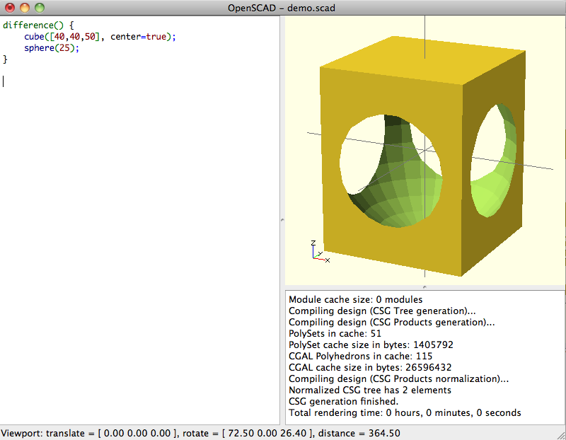
To create a rectangular prism and then take a circle out of the center requires just a few lines of code.
OpenSCAD bills itself as “The Programmers Solid 3D CAD Modeller”. It does this job pretty well, which is probably why I like it so much. Like POV-RAY, which I’ve used before, you create primitive objects–spheres, boxes, cylinders, etc.–and add or subtract them from one another to create the three-dimensional shapes you want.
Unlike the more graphical 3d modeling programs, like SketchUp (which I’ve played with in the past), in OpenSCAD you have to specify in the script the exact dimensions of your primitives, and how to rotate them and translate them to get them where you want them to be in space. This makes it a great language to use in geometry class, or anywhere else you want students to learn about co-ordinate systems.
The script to create the box with a circle cut out of it (see figure above) is:
Vpython requires students of make similar geometric movements of their objects and renders them nicely in 3d, but given the incentive that they can print up a tangible result of their work, I’d be willing to bet that students, especially younger ones, would be quite motivated to work with OpenSCAD. Vpython does retain the advantage that it is able to do animations, while you can only print static objects. In addition, OpenSCAD is more of a scripting language than a programming language like Python (see some of my Vpython programs here).
8th grader models a “fez” he modelled in OpenSCAD. This was the first object, other than the test cube, that was printed on our 3d printer.
The OpenSCAD documentation is quite good. I also found it easy to find instructions on how to create a 3d object from a black and white image, simply by extruding it in the third dimension (by iamwil on the Cubehero Blog and by I Heart Robotics).
One note: I’m using OSX 10.6.8 at the moment, and the current version of OpenSCAD does not work on it. Since I’m loathe to upgrade, I had to use the prior release of OpenSCAD-2013.06.dmg.
On the recommendation of Mr. Schmidt, two of my students have been quite fascinated over the last few days trying to solve problems on Project Euler. They’ve been working on them together to, I suspect, the detriment of some of their other classes, but as their math teacher I find it hard to object.
An example problem is something like this:
If we list all the natural numbers below 10 that are multiples of 3 or 5, we get 3, 5, 6 and 9. The sum of these multiples is 23.
Find the sum of all the multiples of 3 or 5 below 1000.
They’ve been solving them numerically using Python. It’s been quite fascinating to see.
Student’s program to calculate the volume of a curve rotated around the x-axis using the Disk Method in Calculus.
This VPython program was written by a student, Mr. Alex Shine, to demonstrate how to find the volume of a curve that’s rotated around the x-axis using the disk method in Calculus II.
The program finds volume for the curve:
between x = 0 and x = 3.
To change the curve, change the function R(x), and to set the upper and lower bounds change a and b respectively.
volume_disk_method.py by Alex Shine.
from visual import*

def R(x):
    y = -(1.0/4.0)*x**2 + 4
    return y

dx = 0.5

a = 0.0

b = 3.0

x_axis = curve(pos=[(-10,0,0),(10,0,0)])

y_axis = curve(pos=[(0,-10,0),(0,10,0)])

z_axis = curve(pos=[(0,0,-10),(0,0,10)])

line = curve(x=arange(0,3,.1))
line.color=color.cyan
line.radius = .1
line.y = -(1.0/4.0) * (line.x**2) + 4

#scene.background = color.white

for i in range(-10, 11):

    curve(pos=[(-0.5,i),(0.5,i)])
    curve(pos=[(i,-0.5),(i,0.5)])

VT = 0


for x in arange(a + dx,b + dx,dx):

    V = pi * R(x)**2 * dx

    disk = cylinder(pos=(x,0,0),radius=R(x),axis=(-dx,0,0), color = color.yellow)

    VT = V + VT

    print V

print "Volume =", VT
Frequency.
I’ve slapped together this simple VPython program to introduce sinusoidal functions to my pre-Calculus students.
Left and right arrow keys increase and decrease the frequency;
Up and down arrow keys increase and decrease the amplitude;
“a” and “s” keys increase and decrease the phase.
Amplitude.
The specific functions shown on the graph are based on the general function:
where:
A — amplitude
F — frequency
P — phase
Phase. Note how the curve seems to move backward when the phase increases.
When I first introduce sinusoidal functions to my pre-Calculus students I have them make tables of the functions (from -2π to 2π with an interval of π/8) and then plot the functions. Then I’ll have them draw sets of sine functions so they can observe different frequencies, amplitudes, and phases.
from visual import *

class sin_func:
    def __init__(self, x, amp=1., freq=1., phase=0.0):
        self.x = x
        self.amp = amp
        self.freq = freq
        self.phase = phase

        self.curve = curve(color=color.red, x=self.x, y=self.f(x), radius=0.05)
        self.label = label(pos=(xmin/2.0,ymin), text="Hi",box=False, height=30)

    def f(self, x):
        y = self.amp * sin(self.freq*x+self.phase)
        return y

    def update(self, amp, freq, phase):
        self.amp = amp
        self.freq = freq
        self.phase = phase
        self.curve.y = self.f(x)
        self.label.text = self.get_eqn()

    def get_eqn(self):
        if self.phase == 0.0:
            tphase = ""
        elif (self.phase > 0):
            tphase = u" + %i\u03C0/8" % int(self.phase*8.0/pi)
        else:
            tphase = u" - %i\u03C0/8" % int(abs(self.phase*8.0/pi))
        print self.phase*8.0/pi

        txt = "y = %ssin(%sx %s)" % (simplify_num(self.amp), simplify_num(self.freq), tphase)
        return txt

def simplify_num(num):
    if (num == 1):
        snum = ""
    elif (num == -1):
        snum = "-"
    else:
        snum = str(num).split(".")[0]+" "
    return snum

amp = 1.0
freq = 1.0

damp = 1.0
dfreq = 1.0

phase = 0.0
dphase = pi/8.0

xmin = -2*pi
xmax = 2*pi
dx = 0.1

ymin = -3
ymax = 3

scene.width=640
scene.height=480

xaxis = curve(pos=[(xmin,0),(xmax,0)])
yaxis = curve(pos=[(0,ymin),(0,ymax)])

x = arange(xmin, xmax, dx)
#y = f(x)

func = sin_func(x=x)
func.update(amp, freq, phase)

while 1: #theta <= 2*pi:
    rate(60)

    if scene.kb.keys: # is there an event waiting to be processed?
        s = scene.kb.getkey() # obtain keyboard information
        #print s
        if s == "up":
            amp += damp
        if s == "down":
            amp -= damp
        if s == "right":
            freq += dfreq
        if s == "left":
            freq -= dfreq

        if s == "s":
            phase += dphase
        if s == "a":
            phase -= dphase

        func.update(amp, freq, phase)
        #update_curve(func, y)
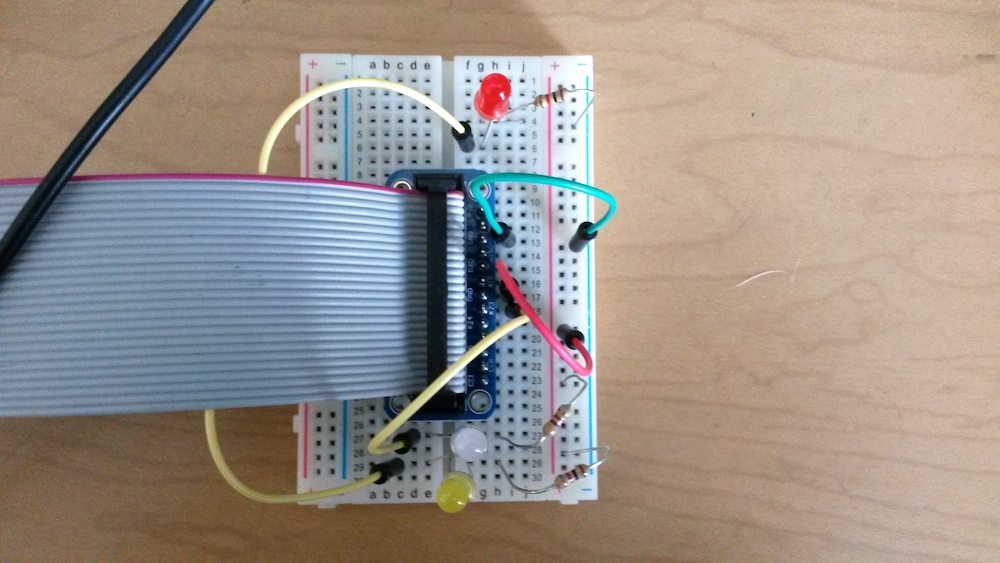
LED light circuits on a breadboard controlled to Raspberry Pi via a cobbler (connected to a ribbon of wires).
Although it took us a day to figure out how to get the Raspberry Pi to work–a faulty SD card turned out to be a major delay–we still had most of a week of the Creativity Interim for students to get some projects done.
That is, until it started to snow. We lost more two days.
Still, we had a small cadre of determined students, one of whom (N.D.) decided that she wanted to make the Pi play sounds to go with the blinking LED lights.
To do this she needed to:
Learn how to use the LINIX command line to connect to the Pi and execute programs.
Learn how to write programs in Python to operate the Pi’s GPIO (input/output) pins.
Learn how to make circuits on a breadboard connected to the Pi.
A Quick and Incomplete Introduction to the Command Line: Basic Navigation
We started by using the Terminal program on my Mac to learn basic navigation.
To see a list of what’s in a folder use ls:
> ls
For more details on the items in the folder, use the -l option:
> ls -l
To see all the options available for the ls command you can lookup the manual using man:
> man ls
To create a new directory (e.g. Pi) use mkdir:
> mkdir Pi
To change directories (say to go into the Pi directory) use cd:
> cd Pi
Connecting to the Pi
I detail how to connect to a Pi that’s plugged into the wall via the local network here, but to summarize:
Use ifconfig to find the local IP address (under eth1).
> ifconfig
Use nmap to identify where the Pi is on the network. E.g.:
> sudo nmap -sP 191.163.3.0/24
Finally, connect to the Pi using the secure shell program ssh:
> ssh pi@191.163.3.214
(the default password is “raspberry”)
Wiring an LED Light Circuit
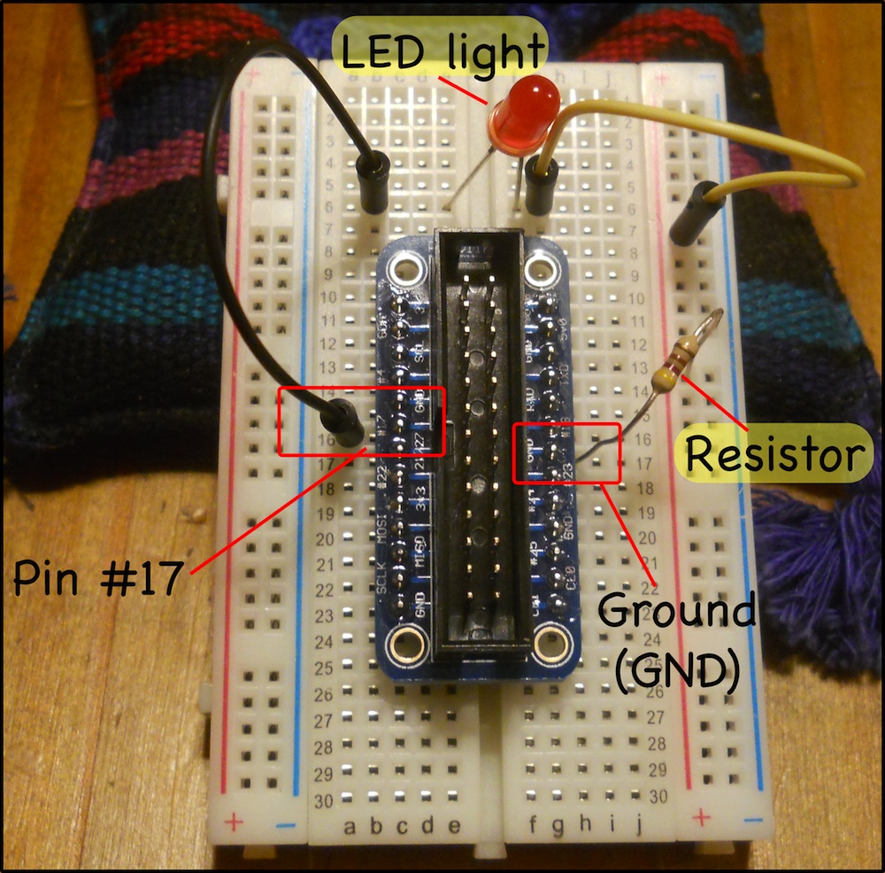
A circuit that connects the #17 GPIO pin to a red LED light then to a resistor before going back into the ground (GND).
We created an initial circuit going from the #17 General Purpose Input/Output (GPIO) pin to a red LED then through a resistor then back into one of the ground pins of the Pi. We’ll turn the current going through GPIO #17 on and off via our program on the Pi. The resistor is needed to reduce the amount of current flowing through the LED, otherwise it would likely get blown out. The circuit is shown in the picture where I’ve taken the wire ribbon out for the sake of visibility.
Wiring on a breadboard is quite simple if you remember a few rules.
First, the columns of holes on the sides are connected vertically, so the right end of the yellow wire (in the + column) is connected to the resistor.
Secondly, the holes in the middle are connected horizontally, but not across the gap in the middle. That’s why the GPIO pin #17 is connected to the lower end of the black wire, and the left end of the resistor is connected to the ground (GND) pin. The LED light reaches across the two gap to connect the two rows with the upper end of the black wire and the left end of the yellow wire. Without something to bridge the gap, the circuit would not be complete.
The resistor has a resistance of 420 Ohms. You can tell by the color bands. In the sequence–yellow, red, brown–the first two bars represent numbers (yellow=4; red=2) and the third number represents a multiplier (in this case brown represents 10x).
Light: Programming the Pi in Python
Once you ssh to the Pi you can start programming. We used the command line text editor Nano. A simple text editor is all you need to write simple Python programs. We’ll create a program called flash.py (Note: it’s important to include the .py at the end of the file’s name, otherwise it becomes hard to figure out what type of file something is, and the extension also clues Nano in to allow it to color-code the keywords used in Python, making it a lot easier to write code.
pi> nano flash.py
You can then type in your program. The basic code for making a single light flash on and off ten times (see here) is:
flash.py
#!/usr/bin/env python

from time import sleep
import RPi.GPIO as GPIO

cpr = 17  ## The GPIO Pin output number

GPIO.setmode(GPIO.BCM) ## Use board pin numbering

GPIO.setup(cpr, GPIO.OUT) ## Setup GPIO Pin 7 to OUT

for i in range(10):
	GPIO.output(cpr, True)
	sleep(0.5)
	GPIO.output(cpr, False)
	sleep(0.5)
GPIO.cleanup()
This requires wiring a circuit to the GPIO pin #17. The circuit has a LED and a resistor in series, and circles back to the Pi via a grounding pin.
Run the program flash.py using:
pi> sudo python flash.py
Finally, let’s tell the program how many times to flash the light. We could create a variable in the Python code with a number, but it’s more flexible to set Python to take the number from the command line as a command line argument. Any words you put after the python in the command to run your program are automatically stored in an array called sys.argv if you import the sys module into your program. So we rewrite our flash.py program as:
flash2.py
#!/usr/bin/env python

from time import sleep
import RPi.GPIO as GPIO
import sys

cpr = 17  ## The GPIO Pin output number

GPIO.setmode(GPIO.BCM) ## Use board pin numbering

GPIO.setup(cpr, GPIO.OUT) ## Setup GPIO Pin 7 to OUT

for i in range(int(sys.argv[1])):
	GPIO.output(cpr, True)
	sleep(0.5)
	GPIO.output(cpr, False)
	sleep(0.5)
GPIO.cleanup()
So to flash the light 8 times use:
pi> sudo python flash2.py 8
Note that in your Python code you use int(sys.argv[1]) to get the number of times to flash:
sys.argv[1] refers to the first word on the command line after the name of the python file. sys.argv[0] would give you the name of the python file itself (flash.py in this case).
the int function converts strings (letters and words) into numbers that Python can understand. When Python reads in the “8” from the command line it treats it like the character “8” rather than the number 8. You need to tell Python that “8” is a number.
Sound: Using SOX
You can do a lot with sound–record, play files, synthesize notes–on the Pi using the command line program SOX. Install SOS (and mplayer and ffmpeg which are necessary as well) using:
pi> sudo apt-get install sox mplayer ffmpeg
Installation may take a while, but when it’s done, if you plug in speakers or headphones–the Pi has no onboard speakers–you can test by synthesizing an E4 note, which has a frequency of 329.63 Hz (via Physics of Music Notes), that lasts for half a second using:
pi> play -n synth .5 sin 329.63
Now play is a command line program that’s part of sox, so to use it in your Python program you have to tell Python to import the module that lets Python talk to the command line: it’s called os. Then you make a Python program to play the note using os.system like so:
test_sound.py
import os
os.system('play -n synth .5 sin 329.63')
And run the program with:
pi> sudo python test_sound.py
Combining light and sound
Now we bring the light and sound together a the Python program:
flash-note.py
#!/usr/bin/env python

from time import sleep
import RPi.GPIO as GPIO
import sys
import os

cpr = 17  ## The GPIO Pin output number

GPIO.setmode(GPIO.BCM) ## Use board pin numbering

GPIO.setup(cpr, GPIO.OUT) ## Setup GPIO Pin 7 to OUT

for i in range(int(sys.argv[1])):
	GPIO.output(cpr, True)
	os.system('play -n synth .5 sin 329.63')
	GPIO.output(cpr, False)
	sleep(0.5)
GPIO.cleanup()
which you run (repeating the note and light 5 times) with:
pi> sudo python flash-note.py 5
Notice that we’ve replaced the middle sleep(0.5) line with the call to play the note because we don’t need the delay since the note plays for 0.5 seconds.
Playing a Tune
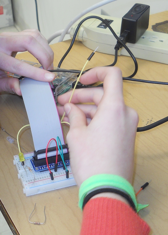
N.D. wires LED’s and resistors on a breadboard connected to a Raspberry Pi.
The student, N.D., spent some time working through this programming and adding wiring to the Pi breadboard in order to play the first few notes of Mary Had A Little Lamb. By the time we ran out of time, and she had to do her presentation to the rest of the upper-school, she’d come up with this:
red-light-flash.py
#!/usr/bin/env python

from time import sleep
import os
import sys
import RPi.GPIO as GPIO
os.system('play -n synth 2 sin 543.21')

cpy = 22
cpr = 17
cpw = 23

GPIO.setmode(GPIO.BCM) ## Use board pin numbering

GPIO.setup(cpy, GPIO.OUT) ## Setup GPIO Pin 0 to OUT
GPIO.setup(cpr, GPIO.OUT)
GPIO.setup(cpw, GPIO.OUT)

for i in range(int(sys.argv[1])):
	GPIO.output(cpy, True)
	GPIO.output(cpr, False)
	GPIO.output(cpw, False)
	os.system('play -n synth 1 sin 578.00')
	GPIO.output(cpy, False)
	GPIO.output(cpr, True)
	GPIO.output(cpw, False)
	os.system('play -n synth 2 sin 440.00')
	GPIO.output(cpy, False)
	GPIO.output(cpr, False)
	GPIO.output(cpw, True)
	os.system('play -n synth 1 sin 400.00')
GPIO.cleanup()
which is run (5 times) using:
pi> sudo python red-light-flash.py 5
Creating User-Defined Functions
(As a note to N.D., because we ran out of time before we could get to it.)
You’ll notice it takes four lines to turn a light on, turn the other lights off, and play the note. You’ll also note that you have to repeat the exact same code every time you want to play a specific note and it becomes a pain having to repeat all this every time, especially if you want to play something with more notes. This is the ideal time to define a function to do all the repetitive stuff.
So we’ll create a separate function for each note. Mary has a little lamb uses the notes E4, D4, and C4. So we get their frequencies from Physics of Music Notes and create the functions:
Another interesting project that came out of the Creativity Interim was a VPython program that uses the DNA Writer translation table to convert text into a DNA sequence that is represented as a series of colored spheres in a helix.
The code, by R.M. with some help from myself, is below. It’s pretty rough but works.
dna_translator.py
from visual import *
import string

xaxis = curve(pos=[(0,0),(10,0)])

inp = raw_input("enter text: ")
inp = inp.upper()


t_table={}


t_table['0']="ATA"
t_table['1']="TCT"
t_table['2']="GCG"
t_table['3']="GTG"
t_table['4']="AGA"
t_table['5']="CGC"
t_table['6']="ATT"
t_table['7']="ACC"
t_table['8']="AGG"
t_table['9']="CAA"
t_table['start']="TTG"
t_table['stop']="TAA"
t_table['A']="ACT"
t_table['B']="CAT"
t_table['C']="TCA"
t_table['D']="TAC"
t_table['E']="CTA"
t_table['F']="GCT"
t_table['G']="GTC"
t_table['H']="CGT"
t_table['I']="CTG"
t_table['J']="TGC"
t_table['K']="TCG"
t_table['L']="ATC"
t_table['M']="ACA"
t_table['N']="CTC"
t_table['O']="TGT"
t_table['P']="GAG"
t_table['Q']="TAT"
t_table['R']="CAC"
t_table['S']="TGA"
t_table['T']="TAG"
t_table['U']="GAT"
t_table['V']="GTA"
t_table['W']="ATG"
t_table['X']="AGT"
t_table['Y']="GAC"
t_table['Z']="GCA"
t_table[' ']="AGC"
t_table['.']="ACG"

dna=""

for i in inp:

    dna=dna+t_table[i]
print dna

m=0
r=3.0
f=0.5
n=0.0
dn=1.5


start_pos = 1
for i in dna:
    rate(10)
    n+=dn
    m+=1
    x = n
    y=r*sin(f*n)
    z=r*cos(f*n)
    a=sphere(pos=(x,y,z))
    #print x, y, z
    if (i == "A"):
        a.color=color.blue
    elif (i== "G"):
        a.color=color.red
    elif (i== "C"):
        a.color=color.green
At higher magnifications, microscope lenses will only be able to focus on layers within your specimen. You could take a series of images with different focal planes and stack them together, but without a camera mounted on the microscope, getting images to line up right for focus stacking is quite the challenge. The alternative is focusing in and out until you get a feeling for the three dimensional shape of the specimen.
Since I don’t have a camera mount I’ve created an html5/javascript page that simulates focusing in and out of a sample. It’s embedded above, but a direct link is here.
You can use the knobs to the right of the image to adjust the focal plane. You should be able to see hairs on the top and bottom of the transparent wing.
One of my students couldn’t get VPython to install and run her computer. She was running Windows 8, and I have not used Windows, much less this version of it to figure out what the problem was. This is one of the challenges with a bring your own device policy. So, instead I gave the lesson on numerical integration using javascript.
If you open the webpage file (index.html) in your browser you should see nothing but the word “Hello”. The template is blank, but it’s ready so students can start with the javascript programming right away, which a few of my programming elective students have done.
For reference, this file (basic-jquery-numeric-int.zip) uses the template to create a program that does numerical integration. Someone using the webpage can enter the limits (a and b) and the number of trapezoids to use (n), and the program calculates calculates the area under the curve f(x) = -x2/4 + x + 4.
It’s a very bare template and doesn’t have any comments, so it’s not useful unless you’re at least a little familiar with html and javascript and just need a clean place to start.