The cold front of this mid latitude cyclone spawned several fatal tornados on April 28, 2011. The cold front is the blue line with triangles pointing toward the east. Image via NOAA HPC.
The cold fronts of mid-latitude cyclones bring thunderstorms, rain and spawn tornadoes like the ones we’ve seen over the last few days. In the spring and fall, these cyclones just sweep across the southern U.S. again and again. The line of their passage sort-of marks the northward migration of the sub-polar low in picture of the global atmospheric circulation system.
The circulation cells of the global atmospheric circulation system migrate north and south with the seasons. Image links to larger version (1 Mb).
Each individual front, with its storms, is a feature of the weather. Climate, on the other hand, is the result of the average position over time: the series of fronts which make the southern U.S. wet in the spring and fall.
The sub-polar low is not the only feature that brings lots of seasonal rain. The ITCZ does also, and the rains that the ITCZ’s movement north and south of the equator bring, are what we call the monsoons. The yellow star on the animation, just to the north of the equator, sees monsoonal rains in the summer. Since the ITCZ follows the sun with the seasons, the monsoons always come in the summer; even in the southern hemisphere.
The first thing you notice is a small, rickety bridge whose main job is to keep your feet dry as you cross a very small stream. The stream is on its delta, so the ground is very soggy, and the channel is just about start its many bifurcations into distributaries that fan out and create the characteristic deltaic shape.
Delta and estuary of the small stream near the villas.
There’s a bright orange flocculate on the quieter parts of the stream bed. It’s the color of fresh rust, which leads me to suspect it’s some sort of iron precipitate.
It is quite easy to stick your finger into the red precipitate at the bottom of the stream.
Iron minerals in the sediments and bedrock of the watershed are dissolved by groundwater, but when that water discharges into the stream it becomes oxygenated as air mixes in. The dissolved iron reacts with the oxygen to create the fine orange precipitate. Sometimes, the chemical reaction is abiotic, other times it’s aided by bacteria (Kadlec and Wallace, 2009).
The bark has been chewed off the top half of this stick. The tooth marks are characteristic of beavers.
Past the small delta, the trail follows the lake as it curves around into another, much bigger estuary (see map above). We found much evidence of flora and fauna, including signs of beavers.
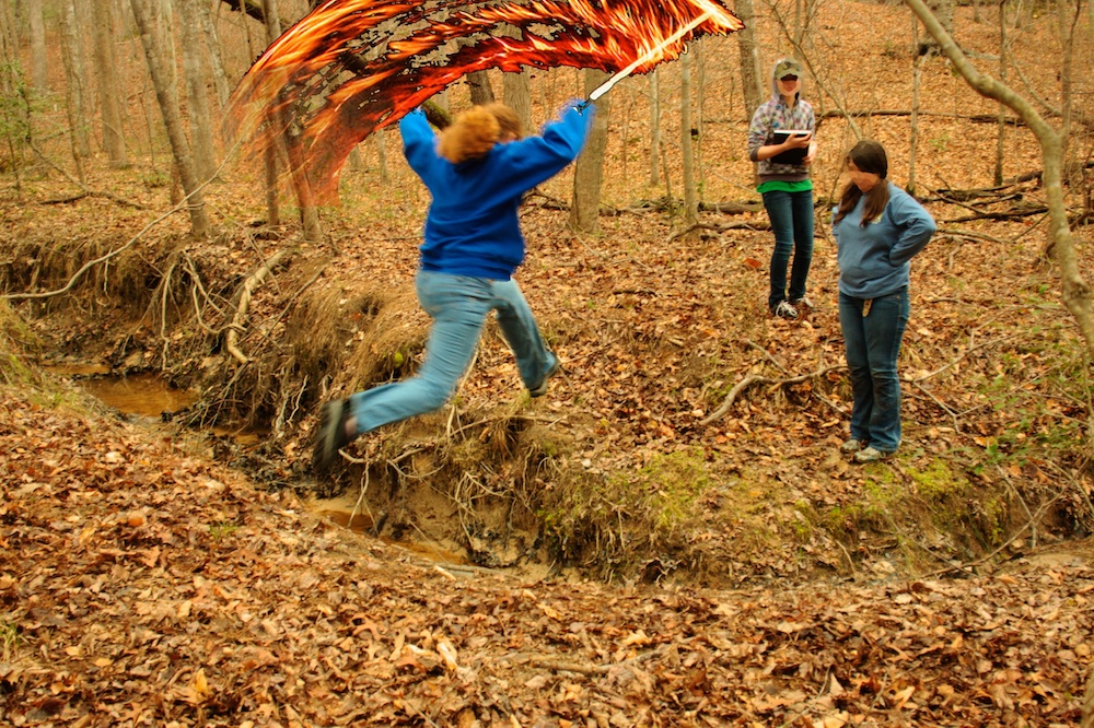
We even took the time to toss some sticks into the water to watch the waves. With a single stick, you can see the wave dissipate as it expands, much like I tried to model for the height of a tsunami. We also threw in multiple sticks to create interference patterns.
Observing interference patterns in waves.
The Oak Ridge Trail, which we followed, diverges from the somewhat longer Pin Oak Trail at the large estuary (which is marked on the map). The Pin Oak Trail takes you through some beautiful stands of conifers, offering the chance to talk about different ecological communities, but we did not have the time to see both trails.
Instead, we followed the Oak Ridge Trail up the ridge (through one small stand of pines) until it met the road. The road is on the other side of the watershed divide. I emphasized the concept by having my students stand in a line across the divide and point in the direction of that a drop of water, rolling across the ground, would flow.
At the watershed divide.
Then I told them that we’d get back by following our fictitious water droplet off the ridge into the valley. And we did, traipsing through the leaf-carpeted woods.
Students imitating water droplets find a dry gully.
Of course there were no water droplets flowing across the surface. Unless its actively raining, water tends to sink down into the soil and flow through the ground until it gets to the bottom of the valley, where it emerges as springs. Even before you see the first spring, though, you can see the gullies carved by overland flow during storms.
Spring.
Following the small stream was quite enjoyable. It was small enough to jump across, and there were some places where the stream had bored short sections of tunnels beneath its bed.
The stream pipes beneath its bed. Jumping up and down over the pipe caused sediment to be expelled at the mouth of the tunnel.
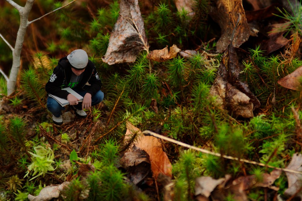
I took the time to observe the beautiful moss that maintained the banks of the stream. Students took the time to observe the environment.
Taking a break at the confluence of two streams.
Downstream the valley got wider and wider, and the stream cut deeper and deeper into the valley floor, but even the small stream sought to meander back and forth, creating beautiful little point bars and cut-banks.
A small, meandering channel. Note the sandy point bars on the inside of the bend, and the overhanging cut-banks on the outside of the curve.
As the stream approached its estuary it would stagnate in places. There, buried leaves and organic matter would decay under the sediment and water in anoxic conditions, rendering their oils and producing natural gas. We’re going to be talking about global warming and the carbon cycle next week so I was quite enthused when students pointed out the sheen of oils glistening on isolated pools of stagnant water.
The breakdown of buried organic matter produces gas and oils that are less dense than water.
Finally, we returned to the estuary. It’s much larger than the first one we saw, and it’s flat, swampy with lots of distributaries, and chock full of the sediment and debris of the watershed above it.
View of the lake from the estuary. The red iron floc in the stream made for a beautiful contrast with the black of the decaying leaves. There is so much red precipitate that it is visible on the satellite image.
This less than three kilometer hike took the best part of two hours. But that’s pretty fast if you value your dawdling.
We’re studying biomes and I don’t know a better way to consider how they’re distributed around the world than by talking about the global atmospheric circulation system. After all, the primary determinants of a biome are the precipitation and temperature of an area.
Diagram showing global atmospheric circulation patterns.
It’s a fairly complicated diagram, but it’s fairly easy to reproduce if you remember a few fairly simple rules: hot air rises; the equator is hotter than the poles; and the Earth rotates out from under the atmosphere.
Hot air rises
Light from the Sun hits the equator directly but hits the poles at a glancing angle, so the equator is warmer than the poles. Warm air at the equator rises while cold air at the poles sinks.
The equator receives more direct radiation from the Sun. A ray of light from the Sun hits the ground at an angle near the poles so it’s spread out more. More radiation at the equator means the ground (or ocean) is warmer, so it warms up the air, which rises.
The warm air can’t rise forever, gravity puts a stop to that. If we did not have gravity the atmosphere would float off into space (and the universe would be a fundamentally different place). Instead, when the air reaches the upper atmosphere at the equator it diverges, heading either north or south toward the poles.
From all around the hemisphere the air converges on the poles. The air is cooling as it moves away from the equator, and when it gets to the pole it sinks to ground level and then makes the journey back to the equator. It’s a cycle, aka a circulation cell.
Hot air rising near the equator and sinking near the poles creates a cycle, a circulation cell, in each hemisphere. In this picture, the winds at ground level (dashed blue lines) would always be blowing from the poles toward the equator. This is what the world might be like without the coriolis effect.
Standing on the ground, the wind would always be blowing towards the equator from the poles. If you were in the northern hemisphere, in say Memphis, you would always be getting northerly winds.
The ITCZ and the Polar High
At the equator the rising air also takes with it water vapor that was evaporated from the oceans or from the land (evaporation and transpiration, which are together called evapotranspiration). The warm air cools as it moves up in the atmosphere and the water vapor forms clouds.
You get a lot of clouds and rainfall anywhere there is a lot of rising air.
Because air is coming together, converging, from north and south at the equator, and the equator is in the middle of the tropics, the zone where you get all this rising air is called the Inter-Tropical Convergence Zone or ITCZ for short (that’s an acronym by the way). The ITCZ is pretty easy to identify from space.
The line of clouds near the equator shows where air is converging at ground level and rising to create clouds. It's called the ITCZ. (Image via NOAA, which also hosts real-time images of the Tropical Atlantic that show the ITCZ very well).
All the rain from the ITCZ, and the warmth of the equator means that when you go looking for tropical rain forests, like the Amazon and the Congo, you’ll find them near the equator.
Locations of rainforests (more or less). Notice that in addition to the Congo and Amazon, Indonesia is pretty well forested too. All because of the ITCZ.
Now at the pole, the air is sinking downward from the upper atmosphere. Sinking air tends to be very dry, and places with sinking air also tend to be dry (it’s not a coincidence). So although the poles are covered with ice, they actually tend to get very little snowfall. What little snow they get tends to accumulate over tens, hundreds and thousands of years but the poles are deserts, arctic deserts, but deserts all the same.
The region of sinking air near the poles is called the polar high because of the high pressure generated by all that descending air.
We’ll complicate the picture of atmospheric circulation now, but the ITCZ and the polar high don’t change.
The Earth Rotates
The complication is the coriolis effect. You see, as the Earth rotates it kind-of drags the atmosphere with it. After all, the atmosphere isn’t nailed down. It’s got it’s own motion and intertia, and doesn’t necessarily want to rotate with the Earth.
Deflection of the wind, represented by a ball, because of the movement of the Earth beneath it. The ball here moves in a straight line but it appears to curve because the Earth is rotating out from under it. Click the image for a bigger, better version.
So a wind blowing from the North pole to the equator gets deflected to it’s right; the northerly wind becomes an easterly.
I could write an entire post about coriolis (and I will) but for now it shall suffice to say that the low-level wind from the pole gets deflected so much that it never reaches the equator. The high-level wind from the equator never reaches the pole, either. Instead of the one, single, circulation cell in each hemisphere, three develop, and you end up with the picture at the top of this post.
In this diagram, the convention is that it shows the circulation cells along the side of the globe, in profile, while the arrows within the circle of the globe show the wind directions on surface.
Note also that the winds in the region just north of the equator (where the label says “Tropical Air”, come from the northeast. These are the northeast trade winds that were vital to the transatlantic trade in the days of sailing ships. Know about them help a lot in the Triangular Trade game.
The Sub-Tropical High and the Sub-Polar Low
With three circulation cells you add the sub-tropical high, and the sub-polar low to the ITCZ and polar high as major features that affect the biomes.
Remember, rising air equals lots of rain, while descending air is dry.
So the sub-tropical high, with its descending air, makes for deserts. Since it’s in the sub-tropics these are hot deserts, the type you typically think about with sand-dunes, camels and dingos.
Sub-tropical deserts from around the world. They're located in the zones 30 degrees north and south of the equator at the sub-tropical high. Base map by Vzb83 via Wikimedia Commons.
The USGS also has a great map that names the major deserts.
Biomes
So if we now look at the map of biomes and climates from around the world we can see the pattern: tropical rainforests near the equator, deserts at 30 degrees north and south, temperate rainforests between 40 and 50 degrees latitude, and arctic deserts at the poles.
Map of biomes from around the world. The different biomes are closely related to the general atmospheric circulation model. (Image adapted from Sten Porse via Wikipedia)
Jonas Bendiksen has an amazing website of photos, sounds and stories from life in slums in South America, Africa and Asia. It’s quite a poignant. You get wide-angled photos from far away and then the photographer steps closer to his subjects until you’re in a panorama of someone’s small apartment, hearing their story.
70 million year old shell and its imprint in a clay matrix, collected at the Coon Creek Science Center.
Collecting the amazingly well-preserved Cretaceous molluscs and arthropods at the Coon Creek Science Center was an excellent way to learn about fossils and the geology of the Mississippi Embayment.
Consider: the actual shell of an actual organism that actually lived 70 million years ago; not the form of the shell, petrified in silica; not the silent imprint of ridges and grooves in the mud of some bivalve’s test, long dissolved by the silent flux of millenia of groundwater flow, although you can find those, too; but to stand in the daylight, on the gravel bar of a creek, and hold the actual shell of an actual marine organism that lived here when it was six meters under water.
When we got to Coon Creek, Pat Broadbent did her typical, excellent presentation, starting with the very basics question of, “What are fossils?” Apart from the aforementioned actual preserved shells, you can also find trace fossils, like, for example, where the imprints of the an organism is left in the mud while the shell itself has long dissolved away. They can be imprints, or molds of the shells. One of my students found the mold of a crab’s claw along the creek bed; the mud filling in the claw had solidified into rock but you could clearly see where the pincer once articulated.
Pat also talked about the Mississippi Embayment, which is the long, broad valley through which the Mississippi River flows.
The breakup of the supercontinent, Pangea. Notice how the North Atlantic Ocean is opening as North America pulls away from Europe and Africa. You can also see the flooded Mississippi Embayment. (Image from Scotese, C.R., 2002, http://www.scotese.com, (PALEOMAP website)).
When the supercontinent Pangea started to break up, North America pulled away from Europe and Africa. This created a rift that eventually became the North Atlantic Ocean. At about the same time, North America tried to split into two as a second rift was created, right where the Mississippi Embayment is today.
How the coastline of North America, has changed over the last 100 million years. The sediments at Coon Creek were deposited in the Cretaceous (black line). The current coastline is shown in blue. (Image from Wikipedia).
But the rift failed (Cox and Van Arsdale, 2007). It did, however, stretch and thin the continental crust enough to create a large inland sea running up the middle of North America. Over the 100 million years since, the rift formed, the Mississippi Embayment has filled in, first with oceanic sediment, but then with terrestrial sands and silts as the mountains to the east and west were eroded away and washed into the inland sea.
The layer of silt and glauconite clay that encases the fossils at Coon Creek is called the Coon Creek Formation. Pat was very clear that we should refer to this material surrounding the fossils as “matrix”. The “d” word was prohibited. These sediments were deposited while the sea still flooded the embayment. They formed a sand bank, several kilometers offshore.
I vaguely remember doing some research on glauconite a long time ago. Glauconite pellets are found in shallow marine waters, usually far enough away from the coastline so that sediment is deposited slowly, and it’s the finer materials, such as silts and clays, that are deposited. The water also needs to be deep enough to protect the fine sediment from the force of the waves. These are ideal conditions for clams, mussels, conchs, and their Cretaceous relatives.
A simple smear of the sediment across a microscope slide is enough to show that the matrix is has a lot of quartz. You need a microscope because the mineral grains are tiny, silt sized or smaller.
But the best part of looking at the slides is finding the microscopic fossils. They’re not as ubiquitous as you might think, but they’re there if you look. I found a couple of forams, a snail-like one and another that looks like a bolivina species.
What looks like a type of bolivina foraminfera. It's benthic, which means that it lives in the sediments not in the water. It is surrounded by silt-sized grains of quartz.
However, the smear slides came later. After Pat’s talk, she took us out to a small mound of matrix that had been excavated for sampling. Everyone grabbed chunks of matrix and pared away at them until they found something promising. These promising samples were wrapped in aluminum foil so we could clean them up under more controlled conditions.
Cleaning samples.
Cleaning takes time and patience, so Pat showed us how to do it, and each student worked on a single sample. The main idea is to create a display of the fossil using the matrix as a base. The general procedure is to:
Use a small pick, paintbrush and spray-bottle of water, to wash and wipe away the matrix from the fossil.
Let it dry out well, which usually takes about five days.
Paint the entire thing with a 50-50 mix of acrylic floor wax and water. Pat recommends Future Floor Wax, but that seems to have been rebranded out of existance.
Repeat that last step three times (let it dry for about 15 minutes inbetween) to get a well preserved, robust sample.
After the instructions on cleaning, we broke for lunch. For most of us lunch could not have come early enough, not because we were particularly hungry, but because it was quite cold outside. Just the week before the temperature had been above 20 °C, t-shirt weather. Now students were clustering around a couple space heaters trying to ward off frostbite (or at least that’s what they claimed). I did offer that they could stay inside after lunch while the rest of the class walked along the creek, but no-one took me up on it. I don’t know if it’s specific to this group or just to adolescents in general, but if there a chance to walk through water, and get dirty and wet, they’ll take it no matter what the consequence.
Students looking for fossils in gravel bar.
Walking the creek, pulling shells and molds out of the gravel bars, was the best part of the visit.
Students standing in the creek, testing their rubber boots.
The water was shallow, not getting up above the shins, despite the rain showers of the preceding days. A few students borrowed rubber boots, which half of them proceeded to fill with water.
There were quite a lot of fossils. Some of the bivalves have really thick strong shells that not only survived the 70 million years since the Cretaceous, but being washed out of the matrix and tumbled down a stream bed with all sorts of sand and gravel. Some of the casts, like the aforementioned arthropod claw, are also pretty robust.
Snail shell that's been in the ground for millions of years and then got washed out into a gravel bar.
A couple of the more interesting finds are the rather elongate tube like structures that are believed to be either fossilized burrows, or fish feces (coporolite). The material in the coporolite has been replaced by minerals, which is why it survived, but it still retains a little of the ick factor.
There’s an awful lot to learn at Coon Creek. I did not even mention the mesosaur skeletons that have been found there, but there is a nice IMAX movie, Sea Monsters, that’s a nice complement to the field trip because it’s set at the same time, and in the same marine environment as the Coon Creek Formation.
Between 6 and 25 km thick, the Earth’s crust is an excruciatingly thin skin on a 6400 km globe. Yet even drilling to the bottom of the crust would require a remarkable feat of engineering. Some geologists want to try.
NPR’s Science Friday interviews Damon Teagle, one of the architects of the project. They want to drill in the ocean because oceanic crust is thinner than continental crust (on the other hand, it’s denser too, which is why it subducts).
Using different types of chocolate covered candy, they also have this wonderful video of the basalts, sheeted dykes and gabbros that make up the crust.
View over the Mississippi River from the scenic outlook in the Trail of Tears State Park. The outlook juts out over rocky bluffs, which allows you to see the flood plain across the river.
Driving through Missouri last week, I stopped at the Trail of Tears State Park, which may be an excellent place to study the post-colonial history of Native Americans (perhaps as part of our civil rights discussions), and observed the Mississippi River and its flood plain before it becomes engorged at its confluence with the Ohio River.
In 1830, President Andrew Jackson passed the Indian Removal Act, which called for the removal of American Indians living east of the Mississippi River to relocate west of the Mississippi River. …
While some of the Cherokees left on their own, more than 16,000 were forced out against their will. In winter 1838-39, an endless procession of wagons, horsemen and people on foot traveled 800 miles west to Indian Territory. Others traveled by boat along river routes. Most of the Cherokee detachments made their way through Cape Girardeau County, home of Trail of Tears State Park. While there, the Indians endured brutal conditions; they dealt with rain, snow, freezing cold, hunger and disease. Floating ice stopped the attempted Mississippi River crossing, so the detachments had to set up camps on both sides of the river. It is estimated that over 4,000 Cherokees lost their lives on the march, nearly a fifth of the population.
Taking a break on the Nature Walk behind the park's museum.
There’s a short, 1 km nature walk behind the building that was nice on a beautiful, sunny day in early spring. Warm, with the trees just barely beginning to bud you can get a feel for the ridge-and-valley topography of the park, which is in stark contrast to the flat floodplain of the Mississippi on the other side of the river. The park’s roads weave up and down the ridges, and I wished I’d had my bike with me.
Barge going downstream on the Mississippi River, past the river-side campground.
This early in the year (mid-March) most of the campgrounds in the interior of the park seem to be closed, but there is one down on a beach of the Mississippi River that was empty but open. This one has electrical hookups which is not a bad thing if you have the place all to yourself.
The scenic outlook is a wooden platform that juts out through the trees so you can see across the Mississippi to the flat floodplain and farmland beyond. Sitting on a cliff of sedimentary rock (it looked like limestone from a distance), the outlook is high enough that you can just make out the shapes of old meander bends and ox-bow lakes.
It’s a small park, probably worth a visit for the museum, and the outlook is nice, but probably not somewhere you’ll want to spend the night unless some of the upland campgrounds are open.
The museum’s focus on the relocation of the Cherokee would be a nice followup to the pre-Columbian focus of the Chucalissa Museum in Memphis.
Cape Girardeau River Wall.
If you’re looking at river processes, you’ll probably also want to stop in Cape Giradeau, which boasts a fromidable wall to protect the downtown from the Mississippi River’s spring floods.
Since we’re working on geometry this cycle, I thought it would be an interesting exercise to think about how we could use geometry to think about how the strength of tsunamis decreases with distance from the source.
Of course, we’ll have to do this using some intense simplification so we can actually apply the tools we have available. The first is to approximate the tsunami as a circular wall of water centered on the epicenter of the earthquake.
Simplified tsunami geometry.
This lets us figure out the volume of the wave pretty easily because we know that the volume of a cylinder is:
(1)
The size of the circular water wall we approximate from the reports from Japan. The maximum height of the wave at landfall was somewhere in the range of 14 m along the northern Japanese coast, which was about 80 km from the epicenter. Just as a wild guess, I’m assuming that the “effective” width of the wave is 1 km.
Typically, in deep water, a tsunami can have a wavelength greater than 500 km (Nelson, 2010; note that our width is half the wavelength), but a wave height of only 1 m (USSRTF). When they reach the shallow water the wave height increases. The Japanese tsunami’s maximum height was reportedly about 14 m.
At any rate, we can figure out the volume of our wall of water by calculating the volume of a cylinder with the middle cut out of it. The radius of our inner cylinder is 80 km, and the radius of the outer cylinder is 80 km plus the width of the wave, which we say here is 1 km.
Calculating the volume of the wave
However, for the sake of algebra, we’ll call the radius of the inner cylinder, ri and the width of the wave as w. Therefore the inner cylinder has a volume of:
(2)
So the radius of the outer cylinder is the radius of the inner cylinder plus the width of the wave:
(3)
which means that the volume of the outer cylinder is:
(4)
So now we can figure out the volume of the wave, which is the volume of the outer cylinder minus the volume of the inner cylinder:
(5)
(6)
Now to simplify, let’s expand the first term on the right side of the equation:
(7)
Now let’s collect terms:
(8)
Take away the inner parentheses:
(9)
and subtract similar terms to get the equation:
(10)
Volume of the wave
Now we can just plug in our estimates of width and height to get the volume of water in the wave. We’re going to assume, later on, that the volume of water does not change as the wave propagates across the ocean.
(11)
rearrange so the coefficients are in front of the variables:
(12)
So, at 80 km, the volume of water in our wave is:
(13)
(14)
Height of the Tsunami
Okay, now we want to know what the height of the tsunami will be at any distance from the epicenter of the earthquake. We’re assuming that the volume of water in the wave remains the same, and that the width of the wave also remains the same. The radius and circumference will certainly change, however.
We take equation (10) and rearrange it to solve for h by first dividing by rearranging all the terms on the right hand side so h is at the end of the equation (this is mostly for clarity):
(15)
Now we can divide by all the other terms on the right hand side to isolate h:
(16)
so:
(17)
which when reversed looks like:
(18)
This is our most general equation. We can use it for any width, or radius of wave that we want, which is great. Anyone else who wants to calculate wave heights for other situations would probably start with this equation (and equation (15)).
Double checking our algebra
So we can now figure out the height of the wave at any radius from the epicenter of the earthquake. To double check our algebra, however, let’s plug in the volume we calculated, and the numbers we started off with, and see if we get the same height (14 m).
First, we’ll use all our initial approximations so we get an equation with only two variables: height (h) and radial distance (ri). Remember our initial conditions:
w = 1000 m
ri = 80,000 m
hi = 14 m
we used these numbers in equation (10) to calculate the volume of water in the wave:
Vw = 7081149841 m3
Now using these same numbers in equation (18) we get:
(19)
which simplifies to:
(20)
So, to double-check we try the radius of 80 km (80,000 m) and we get:
h = 14 m
Aha! it works.
Across the Pacific
Now, what about Hawaii? Well it’s about 6000 km away from the earthquake, so taking that as our radius (in meters of course), in equation (20) we get:
(21)
which is:
h = 0.19 m
This is just 19 cm!
All the way across the Pacific, Lima, Peru, is approximately 9,000 km away, which, using equation (20) gives:
Tsunami heights with distance from earthquake, assuming a circular wall of water.
So the height of the tsunami drops off relatively fast. Within 1000 km of the earthquake the height has dropped by 90%.
How good is this model
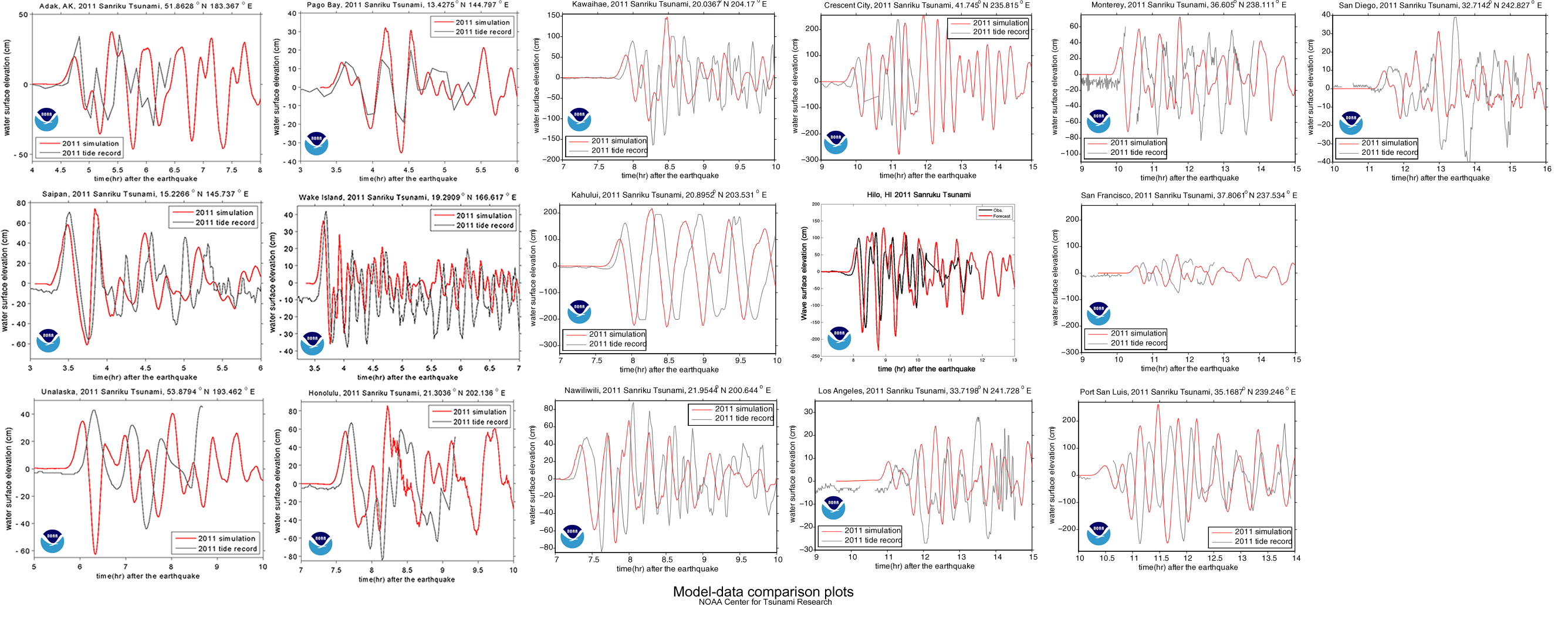
This is all very nice, a cute little exercise in algebra, but is it useful? Does it come anywhere close to reality? We can check by comparing it to actual measurements; the same ones used by NOAA to compare to their model (see here).
The red line is the tsunami's water height predicted by the NOAA computer models for Honolulu, Hawaii, while the black line is the actual water height, measured at a tidal gauge. Other comparisons can be found here. Tsunami wave heights in the Pacific, as modeled by NOAA. Notice how the force of the tsunami is focused across the center of the Pacific.
The graph shows a maximum height of about 60 cm, which is about three times larger than our model. NOAA’s estimate is within 20% of the actual maximum heights, but they’ve spent a bit more time on this problem, so they should be a little better than us. You can find all the gruesome details on NOAA’s Center for Tsunami Research site’s Tsunami Forecasting page.
Notes
1. The maximum height of a tsunami depends on how much up-and-down motion was caused by the earthquake. ScienceDaily reports on a 2007 article that tried to figure out if you could predict the size of a tsunami based on the type of earthquake that caused it.
2. Using buoys in the area, NOAA was able to detect and warn about the Japanese earthquake in about 9 minutes. How do they know where to place the buoys? Plate tectonics.
The locations of the buoys in NOAA's tsunami warning system.
Update
The equations starting with (7) did not have the 2 on the riw term. That has been corrected. Note that the numerical calculations were correct so they have not changed. – Thanks to Spencer and Claude for helping me catch that.


