What are the odds?

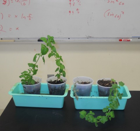
Three successful oregano plants out of four cuttings.

My middle school class stumbled upon a nice probability problem that I might just use in my pre-calculus exam.

Oregano

You see, four of my students took cuttings of oregano plants from the pre-school herb gardens when we were studying asexual reproduction, but only three of them grew roots.

That gives a 75% success rate.

 P[success] = 0.75

The next time I do it, however, I want each student to have some success. If I have them take two cuttings that should increase the chances that at least plant will grow. And we can quantify this.

If the probability of success for each cutting is 75% then the probability of failure is 25%.

P[failure] = 0.25

Given a probability of one plant failing of 25%, the probability of both plants failing is the probability of one plant failing and the other plant failing, which, mathematically, is:

P[2 failures] = P[failure] x P[failure]

P[2 failures] = 0.25 x 0.25

P[2 failures] = 0.252

P[2 failures] = 0.0625

So the probability of at least one plant growing is the opposite of the probability of two failures:

P[at least 1 success of two plants] = 1 – P[2 failures]

P[at least 1 success of two plants] = 1 – 0.0625

P[at least 1 success of two plants] = 0.9375

which is about 94%.

If I had the students plant three cuttings instead, then the probability of at least one success would be:

P[at least 1 success of 3 plants] = 1 – P[3 failures]

P[at least 1 success of 3 plants] = 1 – 0.253

P[at least 1 success of 3 plants] = 1 – 0.02

P[at least 1 success of 3 plants] = 0.98

So 98%.

This means that if I had a class of 100 students then I would expect only two students to not have any cuttings grow roots.

An Equation

In fact, from the work I’ve done here, I can write an equation linking the number of cuttings (let’s call this n) and the probability of success (P). I did this with my pre-calculus class today:

 P = 1 - 0.25^n

so if each student tries 4 cuttings, the probability of success is:

P = 1 – 0.254

P = 1 – 0.004

P = 0.996

Which is 96.6%, which would make me pretty confident that at least one will grow roots.

However, what if I knew the probability of success I needed and then wanted to back calculate the number of plants I’d need to achieve that probability, I could rewrite the equation solving for n:

Start with:
 P = 1 - 0.25^n

isolate the term with n by moving it to the other side of the equation, and switching P as well:
 0.25^n = 1 - P

take the natural log of both sides (we could take the log to the base 10 if we wanted, or any other base log, but ln should work just as well).

 \ln{(0.25^n)} = \ln{(1 - P)}

now use the rules of logarithms to bring the exponent down into a multiplication:

 n \ln{(0.25)} = \ln{(1 - P)}

solving for n gives:

 n  = \frac{\ln{(1 - P)}}{\ln{(0.25)}}

Note that the probability has to be given as a fraction (between 0 and 1), so 90% is P = 0.9. A few of my students made that mistake.

Lavender
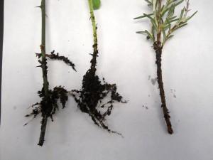
Roots on two of three plants.

At the same time my students were making oregano cuttings, six of them were making cuttings of lavender. Only one of the cuttings grew.

So now I need to find out how many lavender cuttings each student will have to make for me to be 90% sure that at least one of their cuttings will grow roots.

Students can do the math (either by doing the calculations for each step, or by writing and solving the exponential equation you can deduce from the description above), but the graph below shows the results:

Probabilities of successfully growing a lavender cutting.

Graphing Polynomials

Try it. You can change the order and coefficients of the polynomial. The default is the second order polynomial: y = x2.

I originally started putting together this interactive polynomial app to use in demonstrating numerical integration, however it’s a quite useful thing on its own. In fact, I’ve finally figured out how to do iframes, which means that the app is embeddable, so you can use it directly off the Muddle (if you want to put it on your own website you can get the embed code).

This app is a rewritten version of the parabola code, but it uses kineticjs instead of just HTML5 canvases. As a result, it should be much easier to adapt to make it touch/mouse interactive.

Working with Climate Data

Monthly climatic data from the Eads Bridge, from 1893 to the 1960’s. It’s a comma separated file (.csv) that can be imported into pretty much any spreadsheet program.

135045.csv

The last three columns are mean (MMNT), minimum (MNMT), and maximum (MXMT) monthly temperature data, which are good candidates for analysis by pre-calculus students who are studying sinusoidal functions. For an extra challenge, students can also try analyzing the total monthly precipitation patterns (TPCP). The precipitation pattern is not nearly as nice a sinusoidal function as the temperature.

Students should try to deconstruct the curve into component functions to see the annual cycles and any longer term patterns. This type of work would also be a precursor the the mathematics of Fourier analysis.

This data comes from the National Climatic Data Center (NCDC) website.

Rates of change: 4 cm/liter

The first stage rocket booster separates. Image from NASA via Wikipedia.

Fully loaded, the first stage of the Saturn V rockets that launched the Apollo missions would burn through a liter of fuel for every four centimeters it moved. That’s 5 inches/gallon, which, for comparison, is a lot less than your modern automobile that typically gets over 20 miles/gallon.

Ski Trip (to Hidden Valley)

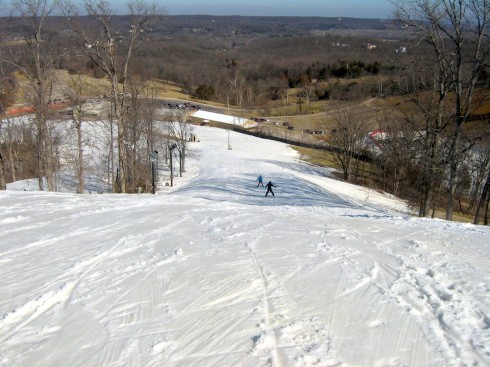
Approaching a change in slope.

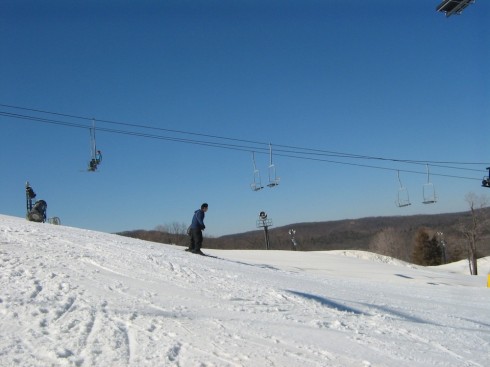
We took a school trip to the ski slopes in Hidden Valley. It was the interim, and it was a day dedicated to taking a break. However, it would have been a great place to talk about gradients, changes in slopes, and first and second differentials. The physics of mass, acceleration, and friction would have been interesting topics as well.

Calculus student about to take the second differential.

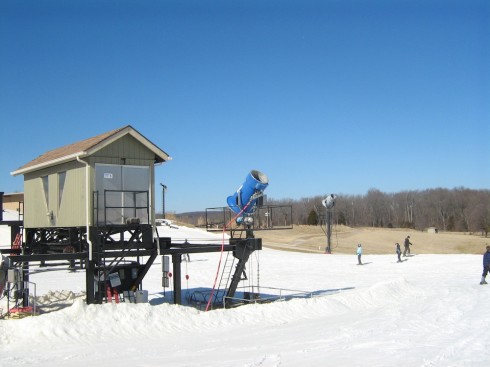
This year has been cooler than last year, but they’ve still struggled a bit to keep snow on the slopes. They make the snow on colder nights, and hope it lasts during the warmer spells. The thermodynamics of ice formation would fit in nicely into physics and discussion of weather, while the impact of a warming climate on the economy is a topic we’ve broached in environmental science already.

The blue cannon launches water into the air, where, if it’s cold enough, it crystallizes into artificial snow. The water is pumped up from a lake at the bottom of the ski slopes.

Influence Explorer: Data on Campaign Contributions by Politician and by Major Contributors

Influence Explorer is an excellent resource for assessing data about money in politics.

The website Influence Explorer has a lot of easily accessible data about the contributions of companies and prominent people to lawmakers. As a resource for civics research it’s really nice, but the time series data also makes it a useful resource for math; algebra and pre-calculus, in particular.

Wiggle Matching: Sorting out the Global Warming Curve

To figure out if the climate is actually warming we need to extract from the global temperature curve all the wiggles caused by other things, like volcanic eruptions and El Nino/La Nina events. The resulting trend is quite striking.

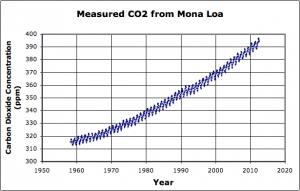
I’m teaching pre-Calculus using a graphical approach, and my students’ latest project is to model the trends in the rising carbon dioxide record in a similar way. They’re matching curves (exponential, parabolic, sinusoidal) to the data and subtracting them till they get down to the background noise.

Carbon dioxide concentration (ppm) measured at the Mona Loa observatory in Hawaii shows exponential growth and a periodic annual variation.