Finding Volumes Using the Disk Method

Mr. Alex Shine's program to calculate the volume of a curve rotated around the x-axis using the Disk Method in Calculus.
Student’s program to calculate the volume of a curve rotated around the x-axis using the Disk Method in Calculus.

This VPython program was written by a student, Mr. Alex Shine, to demonstrate how to find the volume of a curve that’s rotated around the x-axis using the disk method in Calculus II.

The program finds volume for the curve:

 y = -\frac{x^2}{4} + 4

between x = 0 and x = 3.

To change the curve, change the function R(x), and to set the upper and lower bounds change a and b respectively.

volume_disk_method.py by Alex Shine.

from visual import*

def R(x):
    y = -(1.0/4.0)*x**2 + 4
    return y

dx = 0.5

a = 0.0

b = 3.0

x_axis = curve(pos=[(-10,0,0),(10,0,0)])

y_axis = curve(pos=[(0,-10,0),(0,10,0)])

z_axis = curve(pos=[(0,0,-10),(0,0,10)])

line = curve(x=arange(0,3,.1))
line.color=color.cyan
line.radius = .1
line.y = -(1.0/4.0) * (line.x**2) + 4

#scene.background = color.white

for i in range(-10, 11):

    curve(pos=[(-0.5,i),(0.5,i)])
    curve(pos=[(i,-0.5),(i,0.5)])

VT = 0


for x in arange(a + dx,b + dx,dx):

    V = pi * R(x)**2 * dx

    disk = cylinder(pos=(x,0,0),radius=R(x),axis=(-dx,0,0), color = color.yellow)

    VT = V + VT

    print V

print "Volume =", VT

Sine Curves

Frequency.
Frequency.

I’ve slapped together this simple VPython program to introduce sinusoidal functions to my pre-Calculus students.

  • Left and right arrow keys increase and decrease the frequency;
  • Up and down arrow keys increase and decrease the amplitude;
  • “a” and “s” keys increase and decrease the phase.
Amplitude.
Amplitude.

The specific functions shown on the graph are based on the general function:

 y =  A \sin{F x + P}

where:

  • A — amplitude
  • F — frequency
  • P — phase
Phase. Note how the curve seems to move backward when the phase increases.

When I first introduce sinusoidal functions to my pre-Calculus students I have them make tables of the functions (from -2π to 2π with an interval of π/8) and then plot the functions. Then I’ll have them draw sets of sine functions so they can observe different frequencies, amplitudes, and phases.

from visual import *

class sin_func:
    def __init__(self, x, amp=1., freq=1., phase=0.0):
        self.x = x
        self.amp = amp
        self.freq = freq
        self.phase = phase

        self.curve = curve(color=color.red, x=self.x, y=self.f(x), radius=0.05)
        self.label = label(pos=(xmin/2.0,ymin), text="Hi",box=False, height=30)
        
    def f(self, x):
        y = self.amp * sin(self.freq*x+self.phase)
        return y

    def update(self, amp, freq, phase):
        self.amp = amp
        self.freq = freq
        self.phase = phase
        self.curve.y = self.f(x)
        self.label.text = self.get_eqn()

    def get_eqn(self):
        if self.phase == 0.0:
            tphase = ""
        elif (self.phase > 0):
            tphase = u" + %i\u03C0/8" % int(self.phase*8.0/pi)
        else:
            tphase = u" - %i\u03C0/8" % int(abs(self.phase*8.0/pi))
        print self.phase*8.0/pi

        txt = "y = %ssin(%sx %s)" % (simplify_num(self.amp), simplify_num(self.freq), tphase)
        return txt
    
def simplify_num(num):
    if (num == 1):
        snum = ""
    elif (num == -1):
        snum = "-"
    else:
        snum = str(num).split(".")[0]+" "
    return snum
        
amp = 1.0
freq = 1.0

damp = 1.0
dfreq = 1.0

phase = 0.0
dphase = pi/8.0

xmin = -2*pi
xmax = 2*pi
dx = 0.1

ymin = -3
ymax = 3

scene.width=640
scene.height=480

xaxis = curve(pos=[(xmin,0),(xmax,0)])
yaxis = curve(pos=[(0,ymin),(0,ymax)])

x = arange(xmin, xmax, dx)
#y = f(x)

func = sin_func(x=x)
func.update(amp, freq, phase)

while 1: #theta <= 2*pi:
    rate(60)

    if scene.kb.keys: # is there an event waiting to be processed?
        s = scene.kb.getkey() # obtain keyboard information
        #print s
        if s == "up":
            amp += damp
        if s == "down":
            amp -= damp
        if s == "right":
            freq += dfreq
        if s == "left":
            freq -= dfreq

        if s == "s":
            phase += dphase
        if s == "a":
            phase -= dphase

        func.update(amp, freq, phase)
        #update_curve(func, y)
        

Parabolic Trajectories

The post below was contributed by Michael Schmidt, our math teacher.

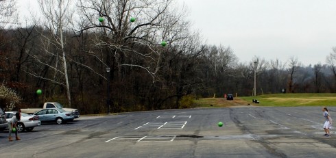
Layered image showing the ballistic path of the green ball thrown by two middle school students. Image by Michael Schmidt.

Parabolas can be a daunting new subject for some students. Often students are not aware of why a parabola may be useful. Luckily, nature always has an answer. Most children realize that a ball thrown through the air will fallow a particular arch but few have made the connected this arch to a parabola. Wonderfully, with a little technology this connection can be made.

With Ms. Hahn’s Canon SLR, I had some of my students throw a ball around outside and took a series of quick pictures of the ball in flight. Since my hand is not very steady, I took the pictures and used the Hugin’s image_stack_align program to align each photo so I could stack them in GIMP.

Within GIMP, I layered the photos on top of each other and cut out the ball from each layer then composed those onto one image. Careful not to move the ball since our later analysis will be less accurate. The result will look something like the following:

Now that there is an image for student to see, we can determine the ball’s height at each point using their own height as a reference. We can then use this information to model a parabola to the data with a site like: http://www.arachnoid.com/polysolve/ .

For the more advanced student an investigation of the least-squares algorithm used by the site may be done.

Now, once we have an expression for the parabola, students can compare how fast they sent the ball into the air.

Experiments for Demonstrating Different Types of Mathematical Functions

This is my quick, and expanding, reference for easy-to-do experiments for students studying different types of functions.

Linear equations: y = mx + b

  • Bringing water to a boil (e.g. Melting snow)
  • Straight line, motorized, motion. (e.g. Movement of a robot/Predicting where robots will meet in the middle)
  • Current versus Voltage across a resistor as resistance changes.

Quadratic equations: y = ax2 + bx + c

Exponential functions: y = aekx

  • Cooling water (ref.)

Square Root Functions: y = ax1/2

Trigonometric Functions: y = asin(bx)+c

Transit

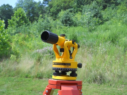
NWI Instruments transit.

This spring I was nominated by my head of school for a small, Teacher of Distinction award offered by the Independent Schools of St. Louis (ISSL). I proposed to get a survey transit that our students could use to map ecological change on campus. My outdoor group has been slowly cutting down the invasive Bradford pear saplings on the slope and I’ve been curious to see if mapping their locations would help us better understand where they’re coming from.

Measuring the distance down to the creek.

The transit would also be a great tool for math. Geometry, algebra, and pre-calculus classes could all benefit because surveying can require quite a bit of geometry and trigonometry.

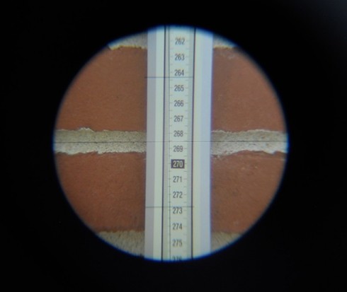
View through the transit.
View through the transit. The middle mark on the reticule allows you to measure elevation change, while the upper and lower marks are used to measure distance. There’s a 100:1 conversion from the distance between the upper and lower marks and the distance from the transit to the measuring rod.

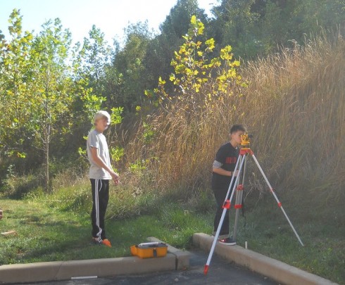
So, I’ve started training a few of my outdoor group in making the measurements. They’ve spent a few weeks learning how to use the transit; we only meet once a week so it goes slowly. However, we’ll start trying to put marks on paper at our next class.

Students trying out the transit.

How much Math do Students Need

Gary Rubinstein argues that we teach too many subjects in math, so we should reduce the number of topics in the curriculum and make math beyond eight grade into electives.

The biggest problem with math education is that there are way too many topics that teachers are required to teach. … When teachers have to teach too many topics, they do not have time to cover them all in a deep way. The teacher, then, has to choose which topics to cover in a meaningful way, and which to cover superficially.

–Rubinstein (2012): The Death of math on Gary Rubinstein’s Blog

And the decision on which subject to cover in-depth is determined by the design of the tests.

I’d certainly support his first suggestion.

The Dish

The Math of Planting Garlic

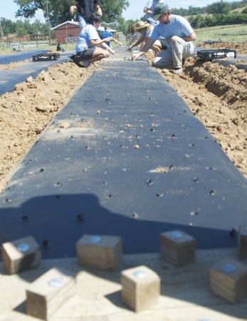
Planting a bed of garlic at the Heifer Ranch CSA.

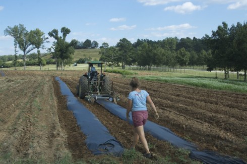
One of the jobs my class helped with at the Heifer Ranch was planting garlic in the Heifer CSA garden. The gardeners had laid rows and rows of this black plastic mulch to keep down the weeds, protect the soil, and help keep the ground warm over the winter.

Laying down the plastic using a tractor. The mechanism simultaneously lays down a drip line beneath the plastic for watering.

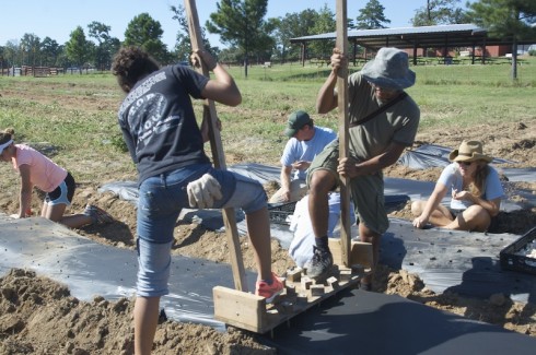
We then used an improvised puncher to put holes in the plastic through which we could plant cloves of garlic pointy side up. The puncher was a simple flat piece of plywood, about one foot by three feet in dimensions, with a set of bolts drilled through. The bolts extended a few inches below the board and would be pressed through the black plastic. Two handles on each side of the board made it easier for two people to maneuver and punch row after row of holes.

Punching holes in the plastic.

As I took my turn punching holes, we did the math to figure out just how much garlic we were planting. A quick count of the last imprint of the puncher showed about 15 holes per punch. Each row was about 200 feet long, which made for approximately 3,000 heads of garlic per row.

We managed to plant one and a half rows. That meant about 4,500 garlic cloves. With ten people planting, that meant each person planted about 450 cloves. Not bad for an afternoon’s work.

Embedding more Graphs (using Flot)

Here’s another attempt to create embeddable graphs of mathematical functions. This one allows users to enter the equation in text form, has the option to enter the domain of the function, and expects there to be multiple functions plotted at the same time. Instead of writing the plotting functions myself I used the FLOT plotting library.